Two-State System

Consider a microscopic system (such as an atom) that possesses two quantum states, labelled 1 and 2. Let the lower energy state, 1 (i.e., the ground state), have energy 0, and let the higher energy state (i.e., the excited state), 2, have energy ${\mit\Delta}$, where ${\mit\Delta}>0$.

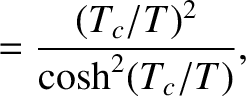
Suppose that the microscopic system is in thermal equilibrium with a heat reservoir of temperature $T$. According to the Boltzmann distribution, (5.329), the probability the system is found in state $i$ is

$$P_i= \frac{\exp(\epsilon_i/k_B\,T)}{\exp(\epsilon_1/k_B\,T)+\exp(-\epsilon_2/k_B\,T)},$$ (5.330)

where $i=1$, $2$. In particular, given that $\epsilon_1=0$ and $\epsilon_2={\mit\Delta}$, we find that

$$P_1 = \frac{1}{1+\exp(-{\mit\Delta}/k_B\,T)},$$ (5.331)

$$P_2\ = \frac{1}{1+\exp({\mit\Delta}/k_B\,T)}.$$ (5.332)

Note that $P_1+P_2=1$. Thus, at low temperatures, $k_B\,T\ll {\mit\Delta}$, we obtain $P_1\rightarrow 1$ and $P_2\rightarrow 0$. In other words, at low temperatures, the system is certain to be found in its ground state, and has no chance of being found in its excited state. On the other hand, at high temperatures, $k_B\,T\gg {\mit\Delta}$, we obtain $P_1=P_2=1/2$. In other words, at high temperatures, the microscopic system is equally likely to be found in its ground state or in its excited state. Finally, the mean energy of the microscopic system is (see Section 5.1.3)

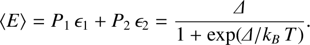$$\langle E\rangle = P_1\,\epsilon_1+P_2\,\epsilon_2 = \frac{{\mit\Delta}}{1+\exp({\mit\Delta}/k_B\,T)} .$$ (5.333)

Note that there is no temperature at which its is possible to get a population inversion; that is, $P_2>P_1$. In fact, lasers, which require a population inversion in order to operate, are not in thermal equilibrium.

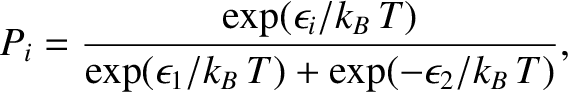
Figure 5.2: Internal energy and specific heat capacity of a two-state system as a function of the temperature.

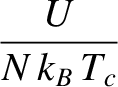
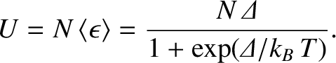
Suppose that we have a macroscopic system consisting of $N$ identical two-state microscopic systems of the type that we have just discussed. The internal energy of the macroscopic system is

$$U= N\,\langle \epsilon\rangle = \frac{N\,{\mit\Delta}}{1+\exp({\mit\Delta}/k_B\,T)}.$$ (5.334)

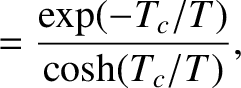
Moreover, the specific heat capacity of the macroscopic system at constant volume is (see Section 5.2.3)

$$C_V = \left(\frac{\partial U}{\partial T}\right)_{V,N} = \frac{N\... ...}{k_B\,T^2}\,\frac{\exp({\mit\Delta}/k_B\,T)}{[1+\exp({\mit\Delta}/k_B\,T)]^2}.$$ (5.335)

The previous two equations yield

$$\frac{U}{N\,k_B\,T_c} = \frac{\exp(-T_c/T)}{\cosh(T_c/T)},$$ (5.336)

$$\frac{C_V}{N\,k_B} = \frac{(T_c/T)^2}{\cosh^2(T_c/T)},$$ (5.337)

where $T_c={\mit\Delta}/(2\,k_B)$. Figure 5.2 illustrates how $U$ and $C_V$ vary with temperature. The peak in the heat capacity is known as the Schottky anomaly, and is associated with the absorption of energy from the heat reservoir as the temperature exceeds the critical temperature required for the constituent microscopic systems to be excited from their ground states.