Next: Exercises
Up: Terrestrial Ocean Tides
Previous: Proudman Equations
Consider a hemispherical ocean for which  and
and
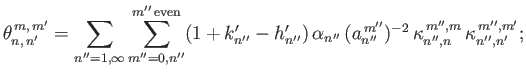
 . In general, there are many linearly independent solutions to
the eigenvalue problem (12.235) and (12.236), subject to the orthonormality constraint (12.244), that correspond to a given value of
. In general, there are many linearly independent solutions to
the eigenvalue problem (12.235) and (12.236), subject to the orthonormality constraint (12.244), that correspond to a given value of  . It is convenient to differentiate these solutions
by means of two indices,
. It is convenient to differentiate these solutions
by means of two indices,  and
and  . Thus,
 and
and
 , where the index
ranges from
, where the index
ranges from  to
to  . Moreover, for
a given value of
, the index
ranges from 0
to
. Now,
. Moreover, for
a given value of
, the index
ranges from 0
to
. Now,
![$\displaystyle \int_0^\pi \cos(m\,\phi)\,\cos(m'\,\phi)\,d\phi =\left\{ \begin{a...
...}&m=m'=0\\ [0.5ex] \pi/2&&m=m'\neq 0\\ [0.5ex] 0&&m\neq m' \end{array} \right..$](img4936.png) |
(12.307) |
Hence, it follows that
 |
(12.308) |
and
 |
(12.309) |
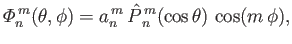
where
![$\displaystyle a_n^{\,m} =\left\{\begin{array}{lll} (4/\lambda_n^{\,m})^{1/2}&\m...
...space{0.5cm}}& m>0\\ [0.5ex] (2/\lambda_n^{\,m})^{1/2}&&m=0 \end{array}\right..$](img4939.png) |
(12.310) |
Likewise, the solutions to the eigenvalue problem (12.248) and (12.249), subject to the orthonormality constraint (12.250), is
such that
 and
and
 , where
 |
(12.311) |
and
 |
(12.312) |
We also have (see Section 12.19)
 |
 |
(12.313) |
 |
 |
(12.314) |
 |
 |
(12.315) |
 |
 |
(12.316) |
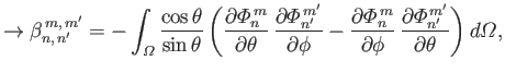
which yields
 |
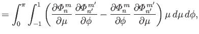 |
(12.317) |
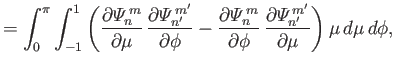
 |
![$\displaystyle = -\int_0^\pi\int_{-1}^{1}\left[(1-\mu^{\,2})\, \frac{\partial{\m...
...}\, \frac{\partial{\mit\Phi}_{n'}^{\,m'}}{\partial\phi}\right]\mu\,d\mu\,d\phi,$](img4951.png) |
(12.318) |
 |
![$\displaystyle = \int_0^\pi\int_{-1}^{1}\left[(1-\mu^{\,2})\, \frac{\partial{\mi...
...\, \frac{\partial{\mit\Psi}_{n'}^{\,m'}}{\partial\phi}\right] \mu\,d\mu\,d\phi,$](img4953.png) |
(12.319) |
 |
 |
(12.320) |
where
 .
However,
.
However,
![$\displaystyle \int_0^\pi \sin(m\,\phi)\,\cos(m'\,\phi)\,d\phi = \left\{ \begin{...
...5cm}} &\mbox{$m+m'$\ odd}\\ [0.5ex] 0&&\mbox{$m+m'$\ even} \end{array}\right. .$](img4956.png) |
(12.321) |
Hence, if  is even then the
 are zero. Otherwise, we
obtain
are zero. Otherwise, we
obtain
 |
 |
(12.322) |
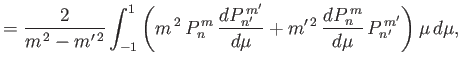
 |
![$\displaystyle =- \frac{2\,m}{m^{\,2}-m'^{\,2}}\int_{-1}^1 \left[(1-\mu^{\,2})\,...
...d\mu} + \frac{m'^{\,2}}{1-\mu^{\,2}}\,P_n^{\,m}\,P_{n'}^{\,m'}\right]\mu\,d\mu,$](img4961.png) |
(12.323) |
 |
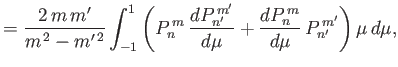 |
(12.324) |
as well as
 |
(12.325) |
where
 |
(12.326) |
Let
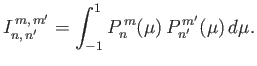 |
(12.327) |
It follows, from symmetry, that
 when
when  is odd.
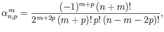
When
is even (Wong 1998),
is odd.
When
is even (Wong 1998),
where
 denotes a gamma function (Abramowitz and Stegun 1965),
 |
(12.328) |
and
![$\displaystyle p_{\rm max} = \left\{ \begin{array}{lll} (n-m)/2&\mbox{\hspace{0....
...\ [0.5ex] (n-m-1)/2&\mbox{\hspace{0.5cm}}&\mbox{$n-m$\ odd} \end{array}\right.,$](img4972.png) |
(12.329) |
with an analogous definition for
 .
.
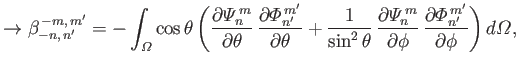
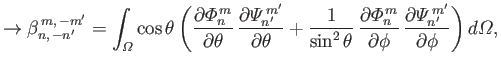
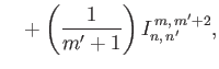
It can be shown that (Longuet-Higgins and Pond 1970)
|
![$\displaystyle = \left[\frac{n'\,(n'+1)+m'\,(m'+1)}{m'+1}-2\,m'\,\frac{n\,(n+1)-n'\,(n'+1)+m'}{m^{\,2}+m'^{\,2}}\right]I_{n,\,n'}^{\,m,\,m'}$](img4974.png) |
|
| |
 |
(12.330) |
 |
 |
|
| |
![$\displaystyle \phantom{\frac{\beta_{n,\,-n'}^{\,m,\,-m'}}{c_n^{\,m}\,c_{n'}^{\,m'}}=} \left.+n'\,(n'+2)\,(n'-m'+1)\,I_{n,\,n'+1}^{\,m,\,m'} \right],$](img4978.png) |
(12.331) |
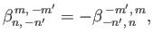
|
 |
(12.332) |
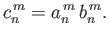
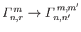
According to Equation (12.306), we can also write
 , where
 |
(12.333) |
and
 |
(12.334) |
Here,
 if
is even, and
if
is even, and
 |
(12.335) |
otherwise.
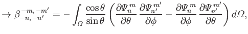
It follows from Equation (12.305) that
 , where
 |
(12.336) |
Here,
 if
is even, and
if
is even, and
 |
(12.337) |
otherwise.
Now, if
and  are both even then
 |
(12.338) |
if
and
are both odd then
 |
(12.339) |
and if
is odd then
 .
.
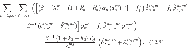
If we let
 and
and
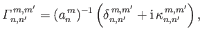
 then Equations (12.311) and (12.312) become
and
 |
(12.340) |
respectively. Here,
 |
 |
(12.341) |
 |
 |
(12.342) |
 |
 |
(12.343) |
 |
 |
(12.344) |
 |
 |
(12.345) |
 |
 |
(12.346) |
 |
 |
(12.347) |
 |
 |
(12.348) |
By symmetry,
 and
and
 are only non-zero when
is even, and
are only non-zero when
is even, and  is even;
 ,
,
 ,
,
 , and
, and
 are
only non-zero when
is odd, and
is odd; and
are
only non-zero when
is odd, and
is odd; and
 and
and
 are only
non-zero when
is odd, and
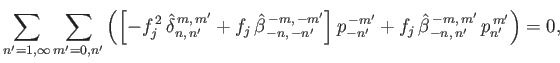
is even. It follows that all quantities appearing in Equations (12.347) and (12.348) are real.
Once we have solved these equations to obtain the
are only
non-zero when
is odd, and
is even. It follows that all quantities appearing in Equations (12.347) and (12.348) are real.
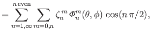
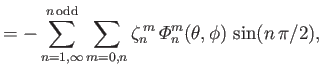
Once we have solved these equations to obtain the  (which is a relatively straightforward numerical task), we can reconstruct the tidal elevation as follows:
 |
(12.349) |
where
and
 |
(12.352) |
Thus, the tidal amplitude at a given point on the ocean is
![$\displaystyle \vert\zeta\vert(\theta,\phi) = \left[\zeta_c^{\,2}(\theta,\phi)+\zeta_s^{\,2}(\theta,\phi)\right]^{1/2}.$](img5028.png) |
(12.353) |
It is easily demonstrated
that
 |
(12.354) |
where
![$\displaystyle {\mit\Delta\varphi}(\theta,\phi) =m_j\,\frac{\pi}{2} + \tan^{-1}\left[\frac{\zeta_s(\theta,\phi)}{\zeta_c(\theta,\phi)}\right].$](img5030.png) |
(12.355) |
Here,
 is the oscillation period of the harmonic of the tide generating potential under consideration,
 is the time-lag between the peak tide
at a given point on the ocean and the maximal tide generating potential at
is the time-lag between the peak tide
at a given point on the ocean and the maximal tide generating potential at
 , and
, and
 is the corresponding phase-lag.
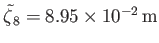
Figures 12.4 and 12.5 show the amplitude and phase-lag of the ( )
)  long-period tide in a hemispherical ocean of
mean depth
long-period tide in a hemispherical ocean of
mean depth
 (which corresponds to
 ), calculated assuming that
 and
and
 .
The calculation includes all azimuthal harmonics up to
.
The calculation includes all azimuthal harmonics up to
 . Note that only a quarter of the ocean is shown, because the amplitude is
symmetric about the meridians
. Note that only a quarter of the ocean is shown, because the amplitude is
symmetric about the meridians
 and
, whereas the phase-lag is
symmetric about the meridian
, and antisymmetric about the meridian
. Here,
and
, whereas the phase-lag is
symmetric about the meridian
, and antisymmetric about the meridian
. Here,
 .
Given that
.
Given that
 (see Table 12.3), the maximum amplitude of the
tide is about
(see Table 12.3), the maximum amplitude of the
tide is about
 , and occurs at the poles. Moreover, it is clear from a comparison with Figure 12.1 that the tide is direct (i.e., it is in phase
with the equilibrium tide).
In fact, the
tide in a hemispherical ocean is about four times larger in amplitude than that in a global ocean (i.e., an ocean that covers the whole surface of the Earth) of the same depth. Otherwise, the two tides have fairly similar properties.
, and occurs at the poles. Moreover, it is clear from a comparison with Figure 12.1 that the tide is direct (i.e., it is in phase
with the equilibrium tide).
In fact, the
tide in a hemispherical ocean is about four times larger in amplitude than that in a global ocean (i.e., an ocean that covers the whole surface of the Earth) of the same depth. Otherwise, the two tides have fairly similar properties.
Figures 12.6 and 12.7 show the amplitude and phase-lag of the ( )
)  diurnal tide in a hemispherical ocean of
mean depth
(which corresponds to
), calculated assuming that
and
.
The calculation includes all azimuthal harmonics up to
.
Given that
diurnal tide in a hemispherical ocean of
mean depth
(which corresponds to
), calculated assuming that
and
.
The calculation includes all azimuthal harmonics up to
.
Given that
 (see Table 12.3), the maximum amplitude of the
tide is about
(see Table 12.3), the maximum amplitude of the
tide is about
 , and occurs at mid-latitudes. This is very different to the case of a global ocean, where the amplitude of the
tide is identically zero everywhere. (See Figure 12.2.)
Note that the tidal phase-lag only exhibits a fairly weak dependence on the azimuthal angle,
, and occurs at mid-latitudes. This is very different to the case of a global ocean, where the amplitude of the
tide is identically zero everywhere. (See Figure 12.2.)
Note that the tidal phase-lag only exhibits a fairly weak dependence on the azimuthal angle,  . In
fact, the
tide in a hemispherical ocean essentially oscillates in anti-phase with the equilibrium tide at the ocean's central longitudinal
meridian (
), except close to the poles, where it oscillates in phase. Again, this is very different to the
case of a global ocean, where the tidal maximum lies on a meridian of longitude, and rotates steadily around the Earth from east to
west.
. In
fact, the
tide in a hemispherical ocean essentially oscillates in anti-phase with the equilibrium tide at the ocean's central longitudinal
meridian (
), except close to the poles, where it oscillates in phase. Again, this is very different to the
case of a global ocean, where the tidal maximum lies on a meridian of longitude, and rotates steadily around the Earth from east to
west.
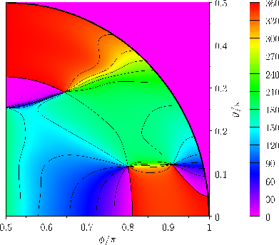
Figures 12.8 and 12.9 show the amplitude and phase-lag of the ( )
)  semi-diurnal tide in a hemispherical ocean of
mean depth
(which corresponds to
), calculated assuming that
and
.
The calculation includes all azimuthal harmonics up to
.
Given that
semi-diurnal tide in a hemispherical ocean of
mean depth
(which corresponds to
), calculated assuming that
and
.
The calculation includes all azimuthal harmonics up to
.
Given that
 (see Table 12.3), the maximum amplitude of the
tide is about
(see Table 12.3), the maximum amplitude of the
tide is about
 , and occurs at the poles. This is very different to the case of a global ocean, where the amplitude of the
tide is zero at the poles. (See Figure 12.3.)
Another major difference is that, in a hemispherical ocean, the tidal maxima circulate around points of zero tidal amplitude--such
points are known as amphidromic points.
Of course, in the case of a global ocean, the tidal maxima lie on opposite meridians of longitude, and rotate steadily around the
Earth from east to west. The systems of tidal waves, circulating around amphidromic points, that is evident in Figure 12.9,
are known as amphidromic systems, and are one of the the major features of tides in real oceans (Cartwright 1999).
Generally speaking, the sense of circulation of amphidromic systems in real oceans is counter-clockwise (seen from above) in the Earth's northern hemisphere, and clockwise
in the southern hemisphere.
, and occurs at the poles. This is very different to the case of a global ocean, where the amplitude of the
tide is zero at the poles. (See Figure 12.3.)
Another major difference is that, in a hemispherical ocean, the tidal maxima circulate around points of zero tidal amplitude--such
points are known as amphidromic points.
Of course, in the case of a global ocean, the tidal maxima lie on opposite meridians of longitude, and rotate steadily around the
Earth from east to west. The systems of tidal waves, circulating around amphidromic points, that is evident in Figure 12.9,
are known as amphidromic systems, and are one of the the major features of tides in real oceans (Cartwright 1999).
Generally speaking, the sense of circulation of amphidromic systems in real oceans is counter-clockwise (seen from above) in the Earth's northern hemisphere, and clockwise
in the southern hemisphere.
In conclusion, our investigation of tides in a hemispherical ocean suggests that the impedance of the flow
of tidal waves around the Earth, due to the presence of the continents, is likely to have a comparatively little effect
on long-period tides, but a very significant effect on diurnal and semi-diurnal tides. In particular, for
semi-diurnal tides, the impedance gives rise to the formation of amphidromic systems.
Figure:
Relative amplitude,
 , of the (
)
long-period tide in a hemispherical ocean.
, of the (
)
long-period tide in a hemispherical ocean.
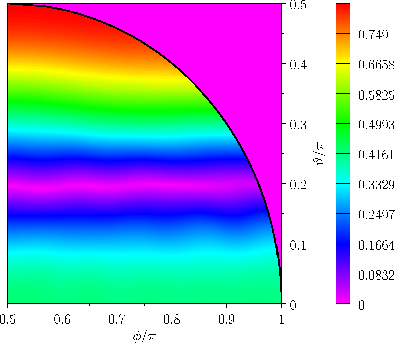 |
Figure:
Phase-lag,
, of the (
)
long-period tide in a hemispherical ocean.
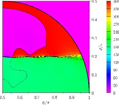 |
Figure:
Relative amplitude,
 , of the (
)
diurnal tide in a hemispherical ocean.
, of the (
)
diurnal tide in a hemispherical ocean.
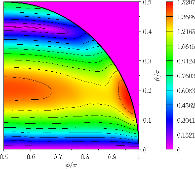 |
Figure:
Phase-lag,
, of the (
)
diurnal tide in a hemispherical ocean.
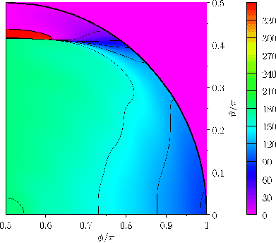 |
Figure:
Relative amplitude,
 , of the (
)
semi-diurnal tide in a hemispherical ocean.
, of the (
)
semi-diurnal tide in a hemispherical ocean.
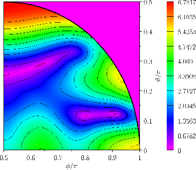 |
Figure:
Phase-lag,
, of the (
)
semi-diurnal tide in a hemispherical ocean.
 |
Next: Exercises
Up: Terrestrial Ocean Tides
Previous: Proudman Equations
Richard Fitzpatrick
2016-03-31
![\begin{multline}
I_{n,\,n'}^{\,m,\,m'} = \sum_{p=0,p_{\rm max}}\sum_{p'=0,p'_{\r...
...)/2]\,{\mit\Gamma}[(m+m'+2p+2p'+2)/2]}{{\mit\Gamma}[(n+n'+3)/2]},
\end{multline}](img4969.png)