Next: Lubrication Theory
Up: Incompressible Viscous Flow
Previous: Taylor-Couette Flow
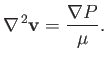
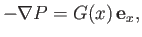
According to Section 10.1, the equations governing steady, incompressible, viscous fluid flow are
As we saw in Sections 10.2 and 10.4, for the case of flow along a straight channel of uniform cross-section,
 and
and
 are both identically zero, and the governing equations consequently reduce to the simple relation
 |
(10.42) |
Suppose, however, that the cross-section of the channel varies along its length. As we shall demonstrate, provided this variation is sufficiently slow, the
flow is still approximately described by the previous relation.
Consider steady, two-dimensional, viscous flow, that is predominately in the  -direction, between two plates that are predominately parallel to
the
-direction, between two plates that are predominately parallel to
the  -
- plane. Let the spacing between the plates,
  , vary on some length scale
  . Suppose that
 |
(10.43) |
where  also varies on the same lengthscale. Assuming that
 and
and
 ,
it follows from Equation (10.40) that
,
it follows from Equation (10.40) that
 |
(10.44) |
Hence,
The
-component of Equation (10.41) reduces to
![$\displaystyle \frac{\partial^{\,2} v_x}{\partial y^{\,2}}\left[1+{\cal O}\left(...
...2}}{\mu\,l}\right)+{\cal O}\left(\frac{d}{l}\right)^2\right] = - \frac{G}{\mu}.$](img3655.png) |
(10.47) |
Thus, if
--in other words, if the channel is sufficiently narrow, and its cross-section varies sufficiently slowly along its length--then Equation (10.47) can be approximated as
 |
(10.50) |
This, of course, is the same as the equation governing steady, two-dimensional, viscous flow between exactly parallel plates. (See Section 10.2.)
Assuming that the plates are located at  and
and  , and making use of the analysis of Section 10.2, the appropriate solution to the previous equation is
![$\displaystyle v_x(x,y) = \frac{G(x)}{2\,\mu}\,y\,[d(x)-y].$](img3662.png) |
(10.51) |
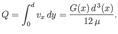
The volume flux (per unit width) of fluid between the plates is thus
 |
(10.52) |
However, for steady incompressible flow, this flux must be independent of
, which implies that
 |
(10.53) |
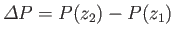
Suppose that a constant difference in effective pressure,
 , is established between the fixed points
  and
and  , where
  .
Integration of the previous equation between these two points yields
.
Integration of the previous equation between these two points yields
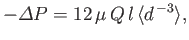 |
(10.54) |
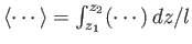
where
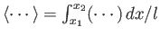 .
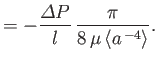
Hence, the volume flux (per unit width) of fluid between the plates that is driven by the effective pressure difference becomes
.
Hence, the volume flux (per unit width) of fluid between the plates that is driven by the effective pressure difference becomes
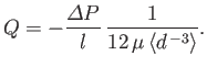 |
(10.55) |
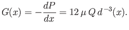
Moreover, the effective pressure gradient at a given point is
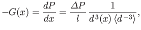 |
(10.56) |
which allows us to determine the velocity profile at that point from Equation (10.51). Thus, given the average effective pressure
gradient,
 , and the variable
separation,
, we can fully specify the flow between the plates.
, and the variable
separation,
, we can fully specify the flow between the plates.
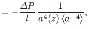
Using analogous arguments to those employed previously, but adapting the analysis of Section 10.4, rather than that of Section 10.1, we can easily show that steady viscous flow down a straight pipe of circular cross-section, whose radius  varies slowly with distance,
, along the pipe, is characterized by
varies slowly with distance,
, along the pipe, is characterized by
Here,  is the volume flux of fluid down the pipe,
 ,
,  , and
, and
 . The approximations used to derive the previous results are valid provided
Next: Lubrication Theory
Up: Incompressible Viscous Flow
Previous: Taylor-Couette Flow
Richard Fitzpatrick
2016-01-22
![$\displaystyle = \frac{\partial^{\,2} v_x}{\partial y^{\,2}}\left[1+{\cal O}\left(\frac{d}{l}\right)^2\right].$](img3654.png)

![$\displaystyle = \frac{G(z)}{4\,\mu}\left[a^{\,2}(z)-r^{\,2}\right],$](img3675.png)