Flow Between Parallel Plates

Consider steady, two-dimensional, viscous flow between two parallel plates that are situated a perpendicular distance $d$ apart. Let $x$ be a longitudinal coordinate measuring distance along the plates, and let $y$ be a transverse coordinate such that the plates are located at $y=0$ and $y=d$ . (See Figure 10.1.)

Figure 10.1: Viscous flow between parallel plates.

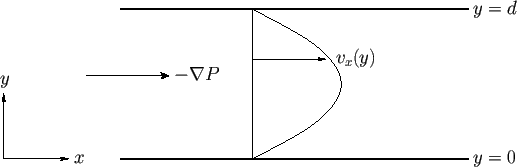Suppose that there is a uniform effective pressure gradient in the $x$ -direction, so that

$$\frac{dP}{dx} =- G,$$ (10.4)

where $G$ is a constant. Here, the quantity $G$ could represent a gradient in actual fluid pressure, a gradient in gravitational potential energy (due to an inclination of the plates to the horizontal), or some combination of the two--it actually makes no difference to the final result. Suppose that the fluid velocity profile between the plates takes the form

$${\bf v} = v_x(y)\,{\bf e}_x.$$ (10.5)

From Section 1.18, this profile automatically satisfies the incompressibility constraint $\nabla\cdot{\bf v}=0$ , and is also such that $D{\bf v}/Dt={\bf0}$ . Hence, Equation (10.2) reduces to

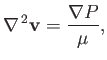$$\nabla^{\,2}{\bf v} = \frac{\nabla P}{\mu},$$ (10.6)

or. taking the $x$ -component,

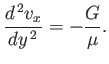$$\frac{d^{\,2} v_x}{dy^{\,2}} = - \frac{G}{\mu}.$$ (10.7)

If the two plates are stationary then the solution that satisfies the no slip constraint (see Section 8.2), 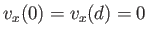$v_x(0)=v_x(d)=0$ , at each plate is

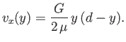$$v_x(y) = \frac{G}{2\,\mu}\,y\,(d-y).$$ (10.8)

Thus, steady, two-dimensional, viscous flow between two stationary parallel plates is associated with a parabolic velocity profile that is symmetric about the midplane, $y=d/2$ . The net volume flux (per unit width in the $z$ -direction) of fluid between the plates is

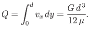$$Q = \int_0^d v_x\,dy = \frac{G\,d^{\,3}}{12\,\mu}.$$ (10.9)

Note that this flux is directly proportional to the effective pressure gradient, inversely proportional to the fluid viscosity, and increases as the cube of the distance between the plates.

Suppose that the upper plate is stationary, but that the lower plate is moving in the $x$ -direction at the constant speed $U$ . In this case, the no slip boundary condition at the lower plate becomes $v_x(0)=U$ , and the modified solution to Equation (10.7) is

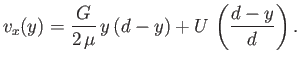$$v_x(y) = \frac{G}{2\,\mu}\,y\,(d-y) + U\,\left(\frac{d-y}{d}\right).$$ (10.10)

Hence, the modified velocity profile is a combination of parabolic and linear profiles. This type of flow is known as Couette flow, in honor of Maurice Couette (1858-1943). The net volume flux (per unit width) of fluid between the plates becomes

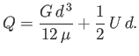$$Q = \frac{G\,d^{\,3}}{12\,\mu}+ \frac{1}{2}\,U\,d.$$ (10.11)