Next: An example 1D PIC
Up: Particle-in-cell codes
Previous: Evaluation of electron number
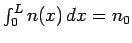
Consider the solution of Poisson's equation:
 |
(303) |
where
 . Note that
  in normalized
units. Let
in normalized
units. Let
 and
and
 .
We can write
.
We can write
which automatically satisfies the periodic boundary conditions  and
and  .
Note that
.
Note that
 , since
 . The other
  are obtained
from
are obtained
from
 |
(306) |
for  .
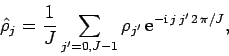
The Fourier transformed version of Poisson's equation yields
.
The Fourier transformed version of Poisson's equation yields
 |
(307) |
and
 |
(308) |
for  , where
 . Finally,
 |
(309) |
for  to
to  , which ensures that the
  remain real.
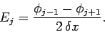
The discretized version of Eq. (297) is
remain real.
The discretized version of Eq. (297) is
 |
(310) |
Of course,  and
and  are special cases which can be resolved using the periodic
boundary conditions.
Finally, suppose that the coordinate of the
are special cases which can be resolved using the periodic
boundary conditions.
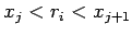
Finally, suppose that the coordinate of the  th electron lies between the
  th and
  th
grid-points: i.e.,
th
grid-points: i.e.,
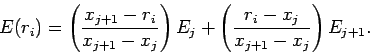
 . We can then use linear interpolation to
evaluate the electric field seen by the th electron:
. We can then use linear interpolation to
evaluate the electric field seen by the th electron:
 |
(311) |
Next: An example 1D PIC
Up: Particle-in-cell codes
Previous: Evaluation of electron number
Richard Fitzpatrick
2006-03-29