Longitudinal Waves on Thin Elastic Rod
Consider a thin uniform elastic rod of length  and cross-sectional area
  .
Let us examine the longitudinal oscillations of such a rod. These oscillations
are often, somewhat loosely, referred to as sound waves. It is again convenient to
let
.
Let us examine the longitudinal oscillations of such a rod. These oscillations
are often, somewhat loosely, referred to as sound waves. It is again convenient to
let  denote position along the rod. Thus, in equilibrium, the
two ends of the rod lie at
denote position along the rod. Thus, in equilibrium, the
two ends of the rod lie at  and
and  . Suppose that a longitudinal wave
causes an -directed displacement
. Suppose that a longitudinal wave
causes an -directed displacement  of the various elements of the rod from their equilibrium positions. Consider a thin section of the rod, of length
  , lying between
 and
and
 . The displacements of the left and right boundaries
of the section are
. The displacements of the left and right boundaries
of the section are
 and
and
 , respectively. Thus, the
change in length of the section, due to the action of the wave, is
, respectively. Thus, the
change in length of the section, due to the action of the wave, is
 . Now,
strain in an elastic rod is defined as change in length over unperturbed
length (Love 1944). Thus, the strain in the section of the rod under consideration is
. Now,
strain in an elastic rod is defined as change in length over unperturbed
length (Love 1944). Thus, the strain in the section of the rod under consideration is
 |
(5.10) |
In the limit
 , this becomes
 |
(5.11) |
It is assumed that the strain is small compared to unity; that is,
 .
Stress,
.
Stress,
 , in an elastic rod is defined as the elastic force
per unit cross-sectional area (ibid.). In a conventional elastic material, the relationship
between stress and strain (for relatively small strains) takes the simple form
, in an elastic rod is defined as the elastic force
per unit cross-sectional area (ibid.). In a conventional elastic material, the relationship
between stress and strain (for relatively small strains) takes the simple form
 |
(5.12) |
Here,  is a constant, with the dimensions of pressure, that is known as the
Young's modulus (ibid.). If the strain in a given element is positive then the stress acts to lengthen the
element, and vice versa. (Similarly, in the spring-coupled mass
system investigated in the preceding section, the external forces exerted on an
individual spring act to lengthen it when its extension is positive, and vice versa.)
is a constant, with the dimensions of pressure, that is known as the
Young's modulus (ibid.). If the strain in a given element is positive then the stress acts to lengthen the
element, and vice versa. (Similarly, in the spring-coupled mass
system investigated in the preceding section, the external forces exerted on an
individual spring act to lengthen it when its extension is positive, and vice versa.)
Consider the motion of a thin section of the rod lying between
and
. If  is the mass density of the rod then the section's mass
is
is the mass density of the rod then the section's mass
is
 . The stress acting on the left boundary of the section
is
. The stress acting on the left boundary of the section
is
 . Because stress is force per
unit area, the force acting on the left boundary is
. Because stress is force per
unit area, the force acting on the left boundary is
 .
This force is directed in the minus -direction, assuming that the strain is positive (i.e., the force acts to lengthen the section). Likewise, the force acting
on the right boundary of the section is
.
This force is directed in the minus -direction, assuming that the strain is positive (i.e., the force acts to lengthen the section). Likewise, the force acting
on the right boundary of the section is
 , and
is directed in the positive -direction, assuming that the strain is positive (i.e., the force again acts to lengthen the section). Finally, the mean longitudinal (i.e., -directed) acceleration of the
section is
, and
is directed in the positive -direction, assuming that the strain is positive (i.e., the force again acts to lengthen the section). Finally, the mean longitudinal (i.e., -directed) acceleration of the
section is
 . Hence, the section's longitudinal equation of motion
becomes
. Hence, the section's longitudinal equation of motion
becomes
![$\displaystyle \rho\,A\,\delta x\,\frac{\partial^{\,2}\psi(x,t)}{\partial t^{\,2}} = A\,Y\left[\epsilon(x+\delta x/2,t)-\epsilon(x-\delta x/2,t)\right].$](img1172.png) |
(5.13) |
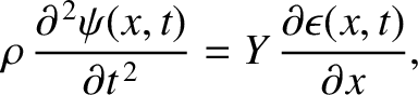
In the limit
, this expression reduces to
 |
(5.14) |
or
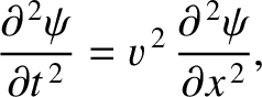 |
(5.15) |
where
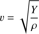 |
(5.16) |
is a constant having the dimensions of velocity, which turns
out to be the propagation speed of longitudinal waves along the rod (see Section 6.2), and
use has been made of Equation (5.11). Equation (5.15) has the same mathematical form as Equation (4.30), which
governs the motion of transverse waves on a uniform string. This implies that
longitudinal and transverse waves in continuous dynamical systems (i.e., systems with an infinite number of degrees of freedom) can be described using the same mathematical
equation.
In order to solve Equation (5.15), we need to specify boundary conditions at the
two ends of the rod. Suppose that the left end of the rod is fixed; that is, it
is clamped in place such that it
cannot move. This implies that
 . Suppose, on the other hand, that
the left end of the rod is free; that is, it is not attached to anything.
This implies that
. Suppose, on the other hand, that
the left end of the rod is free; that is, it is not attached to anything.
This implies that
 , because there is nothing that the end can exert a force (or a stress) on, and vice versa. It follows from Equations (5.11) and (5.12) that
 . Likewise, if the right end of the rod is
fixed then
. Likewise, if the right end of the rod is
fixed then
 , and if the right end is free then
 .
.
Suppose, for the sake of argument, that the left end of the rod is free, and the right
end is fixed. It follows that
, and
.
Let us search for normal modes of the form
 |
(5.17) |
where  ,
,  ,
,  , and
, and  are constants. The
preceding expression automatically satisfies the boundary condition
. The other boundary condition is satisfied provided
are constants. The
preceding expression automatically satisfies the boundary condition
. The other boundary condition is satisfied provided
 |
(5.18) |
which yields
 |
(5.19) |
where  is an integer. As usual, the imposition of the boundary conditions leads
to a quantization of the possible mode wavenumbers.
Substitution of Equation (5.17) into the equation of motion, (5.15), yields the normal mode dispersion relation
is an integer. As usual, the imposition of the boundary conditions leads
to a quantization of the possible mode wavenumbers.
Substitution of Equation (5.17) into the equation of motion, (5.15), yields the normal mode dispersion relation
 |
(5.20) |
The preceding dispersion relation is consistent with the previously derived dispersion relation (5.9), given that
 and
and  . Here,
  is the interplane spacing,
  the mass of a section
of the rod containing a single plane of atoms, and
the mass of a section
of the rod containing a single plane of atoms, and  the effective force constant
between neighboring atomic planes.
the effective force constant
between neighboring atomic planes.
It follows, from the previous analysis, that the th longitudinal normal mode of an elastic rod, of length , whose left end is free, and whose
right end is fixed, is
associated with the characteristic displacement pattern
![$\displaystyle \psi_n(x,t) = A_n\,\cos\left[(n-1/2)\,\pi\,\frac{x}{l}\right]\cos(\omega_n\,t-\phi_n),$](img1186.png) |
(5.21) |
where
 |
(5.22) |
Here,  and
and  are constants that are determined by the initial conditions.
It can be demonstrated that only those normal modes whose mode numbers are positive integers yield unique displacement patterns.
Equation (5.21) describes a standing wave whose nodes (i.e., points where
are constants that are determined by the initial conditions.
It can be demonstrated that only those normal modes whose mode numbers are positive integers yield unique displacement patterns.
Equation (5.21) describes a standing wave whose nodes (i.e., points where  for all
  ) are evenly spaced
a distance
) are evenly spaced
a distance  apart. The boundary condition
ensures that the right end of the rod is always coincident with a node.
On the other hand, the boundary condition
ensures that the left hand of the rod is always coincident with a point of
maximum amplitude oscillation [i.e., a point where
apart. The boundary condition
ensures that the right end of the rod is always coincident with a node.
On the other hand, the boundary condition
ensures that the left hand of the rod is always coincident with a point of
maximum amplitude oscillation [i.e., a point where
 ].
Such a point is known as an anti-node. The anti-nodes associated with a given normal mode lie halfway between the corresponding nodes.
According to Equation (5.22), the normal mode oscillation frequencies depend linearly on
mode number. Finally, it can be shown that, in the long wavelength limit
].
Such a point is known as an anti-node. The anti-nodes associated with a given normal mode lie halfway between the corresponding nodes.
According to Equation (5.22), the normal mode oscillation frequencies depend linearly on
mode number. Finally, it can be shown that, in the long wavelength limit  , the normal modes and normal frequencies of a uniform elastic
rod specified in Equations (5.21) and (5.22) are analogous
to the normal modes and normal frequencies of a linear array of identical spring-coupled masses specified in Equations (5.7) and (5.8), and pictured in
Figures 5.2 and 5.3.
, the normal modes and normal frequencies of a uniform elastic
rod specified in Equations (5.21) and (5.22) are analogous
to the normal modes and normal frequencies of a linear array of identical spring-coupled masses specified in Equations (5.7) and (5.8), and pictured in
Figures 5.2 and 5.3.
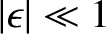
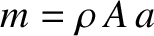
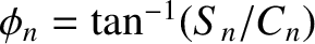
Figure 5.4:
Time evolution of the normalized longitudinal displacement of a thin elastic rod whose left end is free (and is struck with a hammer at  ), and whose right end is fixed. The top-left, top-right, middle-left, middle-right, bottom-left, and bottom-right
panels correspond to
), and whose right end is fixed. The top-left, top-right, middle-left, middle-right, bottom-left, and bottom-right
panels correspond to
 ,
,  ,
,  ,
,  ,
,  ,
,  ,
,  ,
and
,
and  , respectively.
|
|
Because Equation (5.15) is linear, its most general solution
is a linear combination of all of the normal modes; that is,
![$\displaystyle \psi(x,t) = \sum_{n'=1,\infty} A_{n'}\,\cos\left[(n'-1/2)\,\pi\,\frac{x}{l}\right]\,\cos\left[(n'-1/2)\,\pi\,\frac{v\,t}{l}-\phi_{n'}\right].$](img1192.png) |
(5.23) |
The constants and are determined from the initial
displacement,
![$\displaystyle \psi(x,0) = \sum_{n'=1,\infty} A_{n'}\,\cos \phi_{n'}\,\cos\left[(n'-1/2)\,\pi\,\frac{x}{l}\right],$](img1193.png) |
(5.24) |
and the initial velocity,
![$\displaystyle \dot{\psi}(x,0) = \frac{\pi\,v}{l}\sum_{n'=1,\infty} (n'-1/2)\,A_{n'}\,\sin \phi_{n'}\,\cos\left[(n'-1/2)\,\pi\,\frac{x}{l}\right].$](img1194.png) |
(5.25) |
It can be demonstrated that [cf., Equation (4.53)]
![$\displaystyle \frac{2}{l}\int_0^l \cos\left[(n-1/2)\,\pi\,\frac{x}{l}\right]\,\cos\left[(n'-1/2)\,\pi\,\frac{x}{l}\right]dx = \delta_{n,n'}.$](img1195.png) |
(5.26) |
Thus, multiplying Equation (5.24) by
![$(2/l)\,\cos[(n-1/2)\,\pi\,x/l]$](img1196.png) , and integrating in from 0 to , we obtain
, and integrating in from 0 to , we obtain
![$\displaystyle C_n = \frac{2}{l} \int_0^l\psi(x,0)\,\cos\left[(n-1/2)\,\pi\,\frac{x}{l}\right]dx = A_n\,\cos\phi_n,$](img1197.png) |
(5.27) |
where use has been made of Equations (5.26) and (4.54).
Likewise, Equation (5.25) gives
![$\displaystyle S_n =\frac{2}{v\,(n-1/2)\,\pi} \int_0^l\dot{\psi}(x,0)\,\cos\left[(n-1/2)\,\pi\,\frac{x}{l}\right]dx = A_n\,\sin\phi_n.$](img1198.png) |
(5.28) |
Finally,
 and
and
 .
.
Suppose, for the sake of example, that the rod is initially at rest, and that its left end is hit with a hammer at
in such a manner that a section of the rod lying between and  (where
  )
acquires an instantaneous velocity
)
acquires an instantaneous velocity  . It follows that
 .
Furthermore,
.
Furthermore,
 if
if
 , and
, and
 otherwise.
It can be demonstrated that these initial conditions yield
otherwise.
It can be demonstrated that these initial conditions yield  ,
,
 ,
,
![$\displaystyle A_n =S_n= \frac{V_0\,a}{v}\,\frac{2}{\pi}\,\frac{\sin[(n-1/2)\,\pi\,a/l]}{(n-1/2)^{\,2}\,\pi\,a/l},$](img1207.png) |
(5.29) |
and
![$\displaystyle \psi(x,t) = \sum_{n=1,\infty} A_n\,\cos\left[(n-1/2)\,\pi\,\frac{x}{l}\right]\sin\left[(n-1/2)\,\pi\,\frac{t}{\tau}\right],$](img1208.png) |
(5.30) |
where  . Figure 5.4 shows the time evolution of the normalized rod
displacement,
. Figure 5.4 shows the time evolution of the normalized rod
displacement,
 , calculated from the preceding equations using the first 100 normal modes (i.e.,
  ), and choosing
  .
It can be seen that the hammer blow
generates a displacement wave that initially develops at the free end of the rod (
.
It can be seen that the hammer blow
generates a displacement wave that initially develops at the free end of the rod ( ), which is
the end that is struck, propagates along the rod at the velocity
), which is
the end that is struck, propagates along the rod at the velocity  , and reflects off the fixed end (
 ) at time
 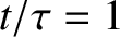 with
no phase shift. (The wave front is traveling from the left to the right in all panels except the final one, where it is traveling from right to left.)
with
no phase shift. (The wave front is traveling from the left to the right in all panels except the final one, where it is traveling from right to left.)
![\includegraphics[width=1\textwidth]{Chapter05/fig5_04.eps}](img1191.png)