Next: Exercises Up: Transverse Standing Waves Previous: Normal Modes of Uniform Contents
 , both ends of
which are attached to immovable walls. These modes are spatially-periodic solutions of the
wave equation, (4.30), that oscillate at unique frequencies and
satisfy the spatial boundary conditions (4.34) and (4.35). Because the wave equation is linear [i.e.,
if
, both ends of
which are attached to immovable walls. These modes are spatially-periodic solutions of the
wave equation, (4.30), that oscillate at unique frequencies and
satisfy the spatial boundary conditions (4.34) and (4.35). Because the wave equation is linear [i.e.,
if  is a solution then so is
 , where
  is an arbitrary constant],
it follows that its most general solution is a linear combination of all of the normal modes.
In other words,
where use has been made of Equations (4.37) and (4.38).
The preceding expression is a solution of Equation (4.30), and also
automatically satisfies the boundary conditions (4.34) and (4.35).
As we have already mentioned, the constants
is an arbitrary constant],
it follows that its most general solution is a linear combination of all of the normal modes.
In other words,
where use has been made of Equations (4.37) and (4.38).
The preceding expression is a solution of Equation (4.30), and also
automatically satisfies the boundary conditions (4.34) and (4.35).
As we have already mentioned, the constants  and
and  are determined
by the initial conditions. Let us see how this comes about in more detail.
are determined
by the initial conditions. Let us see how this comes about in more detail.
Suppose that the initial displacement of the string at  is
is
 |
(4.45) |
 |
(4.46) |
 .
It follows from Equation (4.44) that
.
It follows from Equation (4.44) that
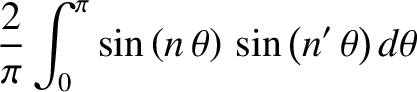
It is readily demonstrated that
where and
and  are (possibly different) positive integers,
 ,
and use has been made of the trigonometric identity
,
and use has been made of the trigonometric identity
 . (See Appendix B.) Furthermore, if
  is a non-zero integer then
 |
(4.50) |
 is a special case, because both the
numerator and the denominator in the preceding expression become zero simultaneously. However, application of l`Hopital's rule yields
is a special case, because both the
numerator and the denominator in the preceding expression become zero simultaneously. However, application of l`Hopital's rule yields
 |
(4.51) |
![\begin{displaymath}\frac{\sin(k\,\pi)}{k\,\pi} = \left\{
\begin{array}{ccc}
1 &\mbox{\hspace{0.5cm}}&k=0\\ [0.5ex]
0&&k\neq 0
\end{array}\right.,\end{displaymath}](img1034.png) |
(4.52) |
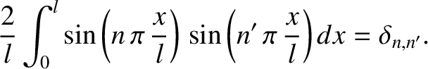
is any integer. This result can be combined with Equation (4.49),
recalling that and are both positive integers, to give
Here, the quantity
where and are integers, is known as the Kronecker delta function.
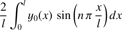
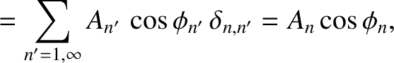
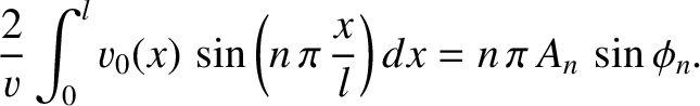
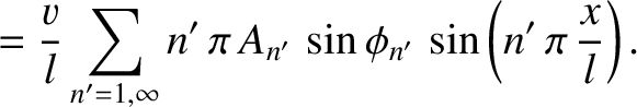
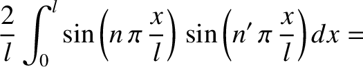
Let us multiply Equation (4.47) by
 , and integrate over
  from 0 to . We obtain
 |
 |
|
 |
(4.55) |
 |
(4.56) |
 , we obtain
 |
 |
(4.59) |
 |
 |
(4.60) |
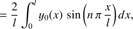
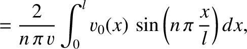
and , appearing in the general expression (4.44) for the time evolution of a uniform string with fixed ends, are
ultimately
determined by integrals over the string's initial displacement and velocity of the form
(4.57) and (4.58).
As an example, suppose that the string is initially at rest, so that
but has the initial displacement This triangular pattern is zero at both ends of the string, rising linearly to the peak value , halfway along the string, and is designed to
mimic the initial displacement of a guitar string that is plucked at its
mid-point. See Figure 4.10.
A comparison of Equations (4.58) and (4.63) reveals that, in this particular example, all of the
, halfway along the string, and is designed to
mimic the initial displacement of a guitar string that is plucked at its
mid-point. See Figure 4.10.
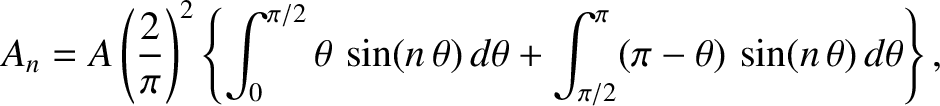
A comparison of Equations (4.58) and (4.63) reveals that, in this particular example, all of the  coefficients
are zero. Hence, from Equations (4.61) and (4.62),
coefficients
are zero. Hence, from Equations (4.61) and (4.62), 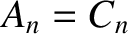 and
and 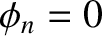 for all . Thus, making use of Equations (4.44), (4.57), and (4.64), the
time evolution of the string is governed by
where
for all . Thus, making use of Equations (4.44), (4.57), and (4.64), the
time evolution of the string is governed by
where
 is the oscillation period of the
  normal mode, and
 |
(4.66) |
 |
(4.67) |
. Integration by parts (Riley 1974) yields
It follows that  whenever is even. We conclude that the triangular initial displacement pattern (4.64) only excites normal modes with odd
mode numbers.
whenever is even. We conclude that the triangular initial displacement pattern (4.64) only excites normal modes with odd
mode numbers.
When a stringed
instrument, such as a guitar, is played, a characteristic pattern of normal
mode oscillations is excited on the plucked string. These oscillations excite
sound waves of the same frequency, which propagate through the air and are audible to a listener.
The normal mode (of appreciable amplitude) with the lowest oscillation
frequency is called the fundamental harmonic, and determines the
pitch of the musical note that is heard by the listener. For instance, a fundamental
harmonic that oscillates at  Hz corresponds to “middle C”. Those normal
modes (of appreciable amplitude) with higher oscillation frequencies than the
fundamental harmonic are called overtone harmonics, because their
frequencies are integer multiples of the fundamental frequency. In general, the
amplitudes of the overtone harmonics are much smaller than the amplitude of the fundamental. Nevertheless, when a stringed instrument is played, the particular mix of overtone harmonics that accompanies the
fundamental determines
the timbre of the musical note heard by the listener. For instance, when middle C
is played on a piano and a harpsichord, the same frequency fundamental harmonic is excited
in both cases. However, the mix of excited overtone harmonics is quite different. This
accounts for the fact that middle C played on a piano can be easily distinguished from middle C
played on a harpsichord.
Hz corresponds to “middle C”. Those normal
modes (of appreciable amplitude) with higher oscillation frequencies than the
fundamental harmonic are called overtone harmonics, because their
frequencies are integer multiples of the fundamental frequency. In general, the
amplitudes of the overtone harmonics are much smaller than the amplitude of the fundamental. Nevertheless, when a stringed instrument is played, the particular mix of overtone harmonics that accompanies the
fundamental determines
the timbre of the musical note heard by the listener. For instance, when middle C
is played on a piano and a harpsichord, the same frequency fundamental harmonic is excited
in both cases. However, the mix of excited overtone harmonics is quite different. This
accounts for the fact that middle C played on a piano can be easily distinguished from middle C
played on a harpsichord.
![\includegraphics[width=0.9\textwidth]{Chapter04/fig4_09.eps}](img1065.png) |
Figure 4.9 shows the ratio  for the first ten overtone harmonics
of a uniform guitar string plucked at its midpoint; that is, the ratio
for odd- modes, with
for the first ten overtone harmonics
of a uniform guitar string plucked at its midpoint; that is, the ratio
for odd- modes, with  , calculated from Equation (4.68). It can be seen that the amplitudes
of the overtone harmonics are all small compared to the amplitude of the
fundamental. Moreover, the amplitudes decrease rapidly in magnitude with increasing
mode number, .
, calculated from Equation (4.68). It can be seen that the amplitudes
of the overtone harmonics are all small compared to the amplitude of the
fundamental. Moreover, the amplitudes decrease rapidly in magnitude with increasing
mode number, .
![\includegraphics[width=0.9\textwidth]{Chapter04/fig4_10.eps}](img1068.png) |
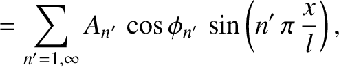
In principle, we must include all of the normal modes in the sum on the right-hand side of Equation (4.65). In practice, given that the amplitudes of the normal
modes decrease rapidly in magnitude as increases, we can truncate the
sum, by neglecting high- normal modes, without introducing significant error
into our calculation. Figure 4.10 illustrates the effect of such a truncation.
In fact, this figure shows the reconstruction of  , obtained by setting
in Equation (4.65), made with various different numbers of normal modes.
It can be seen that sixteen normal
modes is sufficient to very accurately reconstruct the triangular
initial displacement pattern. Indeed, a reconstruction made with only four
normal modes is surprisingly accurate. On the other hand, a reconstruction made
with only one normal mode is fairly inaccurate.
, obtained by setting
in Equation (4.65), made with various different numbers of normal modes.
It can be seen that sixteen normal
modes is sufficient to very accurately reconstruct the triangular
initial displacement pattern. Indeed, a reconstruction made with only four
normal modes is surprisingly accurate. On the other hand, a reconstruction made
with only one normal mode is fairly inaccurate.
![\includegraphics[width=0.9\textwidth]{Chapter04/fig4_11.eps}](img1070.png) |
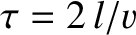
Figure 4.11 shows the time evolution of a uniform guitar
string plucked at its mid-point. It can be seen that the string oscillates in
a rather peculiar fashion. The initial kink in the string at  splits into two
equal kinks that propagate in opposite directions along the string, at the velocity
splits into two
equal kinks that propagate in opposite directions along the string, at the velocity  .
The string remains straight and parallel to the -axis between the kinks, and straight and inclined to the -axis between each kink and the closest wall. When the two
kinks reach the wall, the string is instantaneously found in its undisturbed position. The
kinks then reflect off the two walls, with a phase change of
.
The string remains straight and parallel to the -axis between the kinks, and straight and inclined to the -axis between each kink and the closest wall. When the two
kinks reach the wall, the string is instantaneously found in its undisturbed position. The
kinks then reflect off the two walls, with a phase change of  radians. When the
two kinks meet again at the string is instantaneously found in a state that is an inverted form of its
initial state. The kinks subsequently pass through one another, reflect off the walls, with another phase change of radians, and meet for a second time at . At this
instant, the string is again found in its initial position. The pattern of motion then repeats itself ad infinitum. The period of the oscillation is the time required for a kink to propagate
two string lengths, which is
. This is also the oscillation period of the
normal mode.
radians. When the
two kinks meet again at the string is instantaneously found in a state that is an inverted form of its
initial state. The kinks subsequently pass through one another, reflect off the walls, with another phase change of radians, and meet for a second time at . At this
instant, the string is again found in its initial position. The pattern of motion then repeats itself ad infinitum. The period of the oscillation is the time required for a kink to propagate
two string lengths, which is
. This is also the oscillation period of the
normal mode.


![$\displaystyle \frac{1}{\pi}\int_0^\pi \cos\left[(n-n')\,\theta\right]d\theta$](img1024.png)
![$\displaystyle -\frac{1}{\pi}\int_0^\pi\cos\left[(n+n')\,\theta\right] d\theta$](img1025.png)
![$\displaystyle \frac{1}{\pi}\left[\frac{\sin\left[(n-n')\,\theta\right]}{n-n'}-
\frac{\sin\left[(n+n')\,\theta\right]}{n+n'}\right]_0^{\pi}$](img1026.png)
![$\displaystyle \frac{\sin\left[(n-n')\,\pi\right]}{(n-n')\,\pi}-
\frac{\sin\left[(n+n')\,\pi\right]}{(n+n')\,\pi},$](img1027.png)
![\begin{displaymath}\delta_{n,n'} = \left\{
\begin{array}{ccc}
1 &\mbox{\hspace{0.5cm}}&n=n'\\ [0.5ex]
0&&n\neq n'
\end{array}\right.,\end{displaymath}](img1036.png)


![\begin{displaymath}y_0(x) = 2\,A\left\{
\begin{array}{lcc}
x/l&\mbox{\hspace{0.5...
... x < l/2\\ [0.5ex]
1-x/l &&l/2\leq x\leq l
\end{array}\right. .\end{displaymath}](img1054.png)