Next: General Time Evolution of Up: Transverse Standing Waves Previous: Normal Modes of Beaded Contents
 ,
becomes increasingly large, while the spacing,
,
becomes increasingly large, while the spacing,  , and the individual mass,
  , of the beads become increasingly small. Let the
limit be taken in such
a manner that the length,
, of the beads become increasingly small. Let the
limit be taken in such
a manner that the length,
 , and the average mass per unit length,
 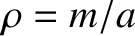 ,
of the string both remain constant. As increases, and becomes very large, such a string will more and
more closely approximate a uniform string of length
,
of the string both remain constant. As increases, and becomes very large, such a string will more and
more closely approximate a uniform string of length  and
mass per unit length
and
mass per unit length  . What can we guess about the normal modes of
a uniform string on the basis of the analysis contained in the preceding section? First of all,
we would guess that a uniform string is an infinite degree of freedom system,
with an infinite number of unique normal modes of oscillation. This follows because a uniform string is the
. What can we guess about the normal modes of
a uniform string on the basis of the analysis contained in the preceding section? First of all,
we would guess that a uniform string is an infinite degree of freedom system,
with an infinite number of unique normal modes of oscillation. This follows because a uniform string is the
 limit of a beaded string, and
a beaded string possesses unique normal modes. Next, we would
guess that the normal modes of a uniform string exhibit smooth sinusoidal spatial variation in the
limit of a beaded string, and
a beaded string possesses unique normal modes. Next, we would
guess that the normal modes of a uniform string exhibit smooth sinusoidal spatial variation in the  -direction, and that the angular frequency of the modes is directly proportional to
their wavenumber. These last two conclusions follow because all of the normal modes of a beaded string are characterized by
-direction, and that the angular frequency of the modes is directly proportional to
their wavenumber. These last two conclusions follow because all of the normal modes of a beaded string are characterized by 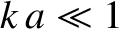 , in the limit in which the spacing between the beads becomes zero. Let us see whether these guesses are correct.
Consider the transverse oscillations of a uniform string of length and mass
per unit length that is stretched between two immovable walls.
It is again convenient to define a Cartesian coordinate system in which
measures distance along the string from the left wall, and  measures
the transverse displacement of the string. Thus, the instantaneous state of the
system at time
measures
the transverse displacement of the string. Thus, the instantaneous state of the
system at time  is determined by the function
  for
for
 .
This function consists of an infinite number of different values,
corresponding to the infinite number of different values in the range 0 to .
Moreover, all of these values are free to vary independently of one another.
It follows that we are indeed dealing with a dynamical system possessing an infinite number
of degrees of freedom.
.
This function consists of an infinite number of different values,
corresponding to the infinite number of different values in the range 0 to .
Moreover, all of these values are free to vary independently of one another.
It follows that we are indeed dealing with a dynamical system possessing an infinite number
of degrees of freedom.
Let us try to reuse some of the analysis of the previous section. We can reinterpret
 as ,
as ,
 as
as
 , and
, and
 as
as
 , assuming that
  and
and
 . Moreover,
 becomes
 ; namely, a second derivative of
with respect to at constant . Finally,
; namely, a second derivative of
with respect to at constant . Finally,
 , where
 is the tension in the string, can be rewritten as
![$T/[\rho\,(\delta x)^{\,2}]$](img976.png) , because
, because
 . Incidentally, we are again assuming that the transverse displacement of the
string remains sufficiently small that the tension is approximately constant in .
Thus, the equation of motion of the beaded string, (4.8), transforms into
. Incidentally, we are again assuming that the transverse displacement of the
string remains sufficiently small that the tension is approximately constant in .
Thus, the equation of motion of the beaded string, (4.8), transforms into
in at constant (see Appendix B), we obtain
 |
(4.27) |
 |
(4.28) |
![$\displaystyle \left[\frac{y(x-\delta x,t)-2\,y(x,t)+y(x+\delta x,t)}{(\delta x)...
...}}\right]
=\frac{\partial^{\,2} y(x,t)}{\partial x^{\,2}} + {\cal O}(\delta x).$](img981.png) |
(4.29) |
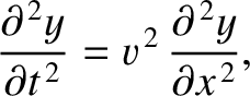
 , Equation (4.26) reduces
to
where
, Equation (4.26) reduces
to
where
 |
(4.31) |
 turns out to be the propagation
velocity of transverse waves along the string. (See Section 6.2.)
turns out to be the propagation
velocity of transverse waves along the string. (See Section 6.2.)
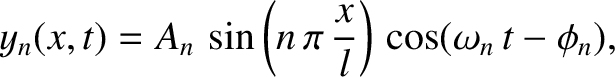
By analogy with Equation (4.12), let us search for a solution of the wave equation of the form
where ,
,  ,
,  , and
, and  are constants. We can interpret such
a solution as a standing wave of wavenumber
are constants. We can interpret such
a solution as a standing wave of wavenumber  , wavelength
 , angular frequency
  ,
peak amplitude
,
peak amplitude  , and phase angle . Substitution of the preceding
expression into Equation (4.30) yields the dispersion relation
[cf., Equation (4.16)]
, and phase angle . Substitution of the preceding
expression into Equation (4.30) yields the dispersion relation
[cf., Equation (4.16)]
 |
(4.33) |
The standing wave solution (4.32) is subject to the physical constraint that the two ends of the string, which are both attached to immovable walls, remain stationary. This leads directly to the spatial boundary conditions
It can be seen that the solution (4.32) automatically satisfies the first boundary condition. However, the second boundary condition is only satisfied when ,
which immediately implies that
,
which immediately implies that
 |
(4.36) |
 , is an integer. We, thus, conclude that the
possible normal modes of a taut string, of length and
fixed ends, have wavenumbers which are quantized such that they
are integer multiples of
, is an integer. We, thus, conclude that the
possible normal modes of a taut string, of length and
fixed ends, have wavenumbers which are quantized such that they
are integer multiples of  . Moreover, this quantization is a direct
consequence of the imposition of the physical boundary
conditions at the two ends of the string.
. Moreover, this quantization is a direct
consequence of the imposition of the physical boundary
conditions at the two ends of the string.
It follows, from the previous analysis, that the th normal mode of the string
is associated with the pattern of motion
 and
and  are constants that are determined
by the initial conditions. (See Section 4.4.) How many unique normal modes are there? The choice
are constants that are determined
by the initial conditions. (See Section 4.4.) How many unique normal modes are there? The choice  yields
 for all and , so this is not a real normal mode. Moreover,
 |
 |
(4.39) |
 |
 |
(4.40) |
 and
and
 . We conclude that
modes with negative mode numbers give rise to the same patterns of motion
as modes with corresponding positive mode numbers. However, modes with
different positive mode numbers correspond to unique patterns of motion that
oscillate at unique frequencies. It follows that the string possesses an infinite number
of normal modes, corresponding to the mode numbers
. We conclude that
modes with negative mode numbers give rise to the same patterns of motion
as modes with corresponding positive mode numbers. However, modes with
different positive mode numbers correspond to unique patterns of motion that
oscillate at unique frequencies. It follows that the string possesses an infinite number
of normal modes, corresponding to the mode numbers  et cetera.
Recall that we are dealing with an infinite-degree-of-freedom system, which
we would expect to possess an infinite number of unique normal modes. The fact that
we have actually obtained an infinite number of such modes suggests that we have found all
of the normal modes.
et cetera.
Recall that we are dealing with an infinite-degree-of-freedom system, which
we would expect to possess an infinite number of unique normal modes. The fact that
we have actually obtained an infinite number of such modes suggests that we have found all
of the normal modes.
![\includegraphics[width=1\textwidth]{Chapter04/fig4_06.eps}](img998.png) |
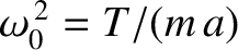
Figure 4.6 illustrates the spatial variation of the first eight normal modes of a uniform string with fixed ends. It can be seen that the modes are all smoothly-varying sine waves. The low-mode-number (i.e., long-wavelength) modes are actually quite similar in form to the corresponding normal modes of a uniformly-beaded string. (See Figure 4.3.) However, the high-mode-number modes are substantially different. We conclude that the normal modes of a beaded string are similar to those of a uniform string, with the same length and mass per unit length, provided that the wavelength of the mode is much larger than the spacing between the beads.
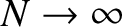
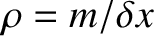
![\includegraphics[width=0.9\textwidth]{Chapter04/fig4_07.eps}](img999.png) |
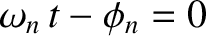
Figure 4.7 illustrates the temporal variation of the  normal mode of
a uniform string. All points on the string attain their maximal
transverse displacements, and pass through zero displacement, simultaneously.
Moreover, the mode possesses five nodes (i.e., points where the string remains stationary). Two of these
are located at the ends of the string, and three in the middle. In fact, according to Equation (4.37), the nodes correspond to points where
normal mode of
a uniform string. All points on the string attain their maximal
transverse displacements, and pass through zero displacement, simultaneously.
Moreover, the mode possesses five nodes (i.e., points where the string remains stationary). Two of these
are located at the ends of the string, and three in the middle. In fact, according to Equation (4.37), the nodes correspond to points where
![$\sin [n\,(x/l)\,\pi]=0$](img1001.png) . Hence, the nodes are located at
. Hence, the nodes are located at
 |
(4.41) |
 is an integer lying in the range 0 to . Here, indexes the normal mode,
and the node. Thus, the
is an integer lying in the range 0 to . Here, indexes the normal mode,
and the node. Thus, the  node lies at the left end of the string, the
 node is the next node to the right, et cetera. It is apparent, from the preceding
formula, that the th normal mode has
node is the next node to the right, et cetera. It is apparent, from the preceding
formula, that the th normal mode has  nodes that are uniformly
spaced a distance
nodes that are uniformly
spaced a distance  apart.
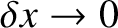
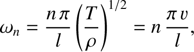
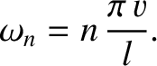
Finally, Figure 4.8 shows the first eight normal frequencies of a uniform string with fixed ends, plotted as a function of the mode number. It can be seen that the angular frequency of oscillation increases linearly with the mode number. Recall that the low-mode-number (i.e., long-wavelength) normal modes of a beaded string also exhibit a linear relationship between normal frequency and mode number of the form [see Equation (4.25)]
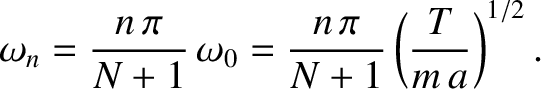 |
(4.42) |
 and
, so we obtain
and
, so we obtain
 |
(4.43) |
![$\displaystyle \frac{\partial^{\,2} y(x,t)}{\partial t^{\,2}} = \frac{T}{\rho}\left[\frac{y(x-\delta x,t)-2\,y(x,t)+y(x+\delta x,t)}{(\delta x)^{\,2}}\right].$](img978.png)


![\includegraphics[width=0.9\textwidth]{Chapter04/fig4_08.eps}](img1008.png)