


Next: Exercises
Up: Quantum Dynamics
Previous: Ehrenfest Theorem
Consider the motion of a particle
in three dimensions in the Schrödinger picture. The fixed dynamical variables of
the system are the position operators,
 , and the momentum operators,
 .
The state of the system is represented as some time evolving ket
.
The state of the system is represented as some time evolving ket
 .
.
Let
 represent a simultaneous eigenket of the position operators
belonging to the eigenvalues
represent a simultaneous eigenket of the position operators
belonging to the eigenvalues
 . Note that, because
the position operators are fixed in the Schrödinger picture, we do not
expect the
. Note that, because
the position operators are fixed in the Schrödinger picture, we do not
expect the
 to evolve in time. The wavefunction of the system
at time
to evolve in time. The wavefunction of the system
at time  is defined
 |
(267) |
The Hamiltonian of the system is taken to be
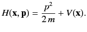 |
(268) |
The Schrödinger equation of motion, (229), yields
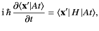 |
(269) |
where use has been made of the time independence of the
.
We adopt the Schrödinger representation in which the momentum conjugate
to the position operator  is written [see Equation (165)]
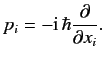 |
(270) |
Thus,
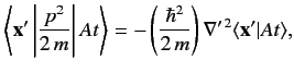 |
(271) |
where use has been made of Equation (169). Here,
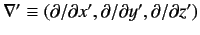 denotes the gradient operator written
in terms of the position eigenvalues. We can also
write
denotes the gradient operator written
in terms of the position eigenvalues. We can also
write
 |
(272) |
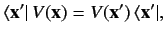
where
 is a scalar function of the position eigenvalues. Combining
Equations (268), (269), (271), and (272), we obtain
is a scalar function of the position eigenvalues. Combining
Equations (268), (269), (271), and (272), we obtain
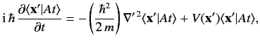 |
(273) |
which can also be written
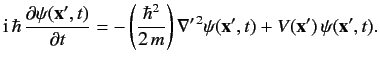 |
(274) |
This is Schrödinger's famous wave equation, and is the basis of
wave mechanics. Note, however, that the wave equation is
just one of many possible representations of quantum mechanics. It just happens
to give a type of equation that we know how to solve. In deriving the wave equation, we have chosen to represent the system in terms of the eigenkets of
the position operators, instead of those of the momentum operators. We have
also fixed the relative phases of the
according to
the Schrödinger representation, so that Equation (270) is valid. Finally, we
have chosen to work in the Schrödinger picture, in which state kets evolve
and dynamical variables are fixed, instead of the Heisenberg picture,
in which the opposite is true.
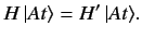
Suppose that the ket
is an eigenket of the Hamiltonian
belonging to the eigenvalue  : i.e.,
 |
(275) |
The Schrödinger equation of motion, (229), yields
 |
(276) |
This can be integrated to give
![$\displaystyle \vert At\rangle = \exp[ -{\rm i}\,H'(t-t_0)/\hbar]\, \vert At_0\rangle.$](img632.png) |
(277) |
Note that
only differs from
 by a phase-factor. The direction of the vector remains fixed in ket space. This
suggests that if the system is initially in an eigenstate of the
Hamiltonian then it remains in this state for ever, as long as the system
is undisturbed. Such a state is called a stationary state. The wavefunction
of a stationary state satisfies
by a phase-factor. The direction of the vector remains fixed in ket space. This
suggests that if the system is initially in an eigenstate of the
Hamiltonian then it remains in this state for ever, as long as the system
is undisturbed. Such a state is called a stationary state. The wavefunction
of a stationary state satisfies
![$\displaystyle \psi({\bf x}', t) = \psi({\bf x'}, t_0) \exp[ -{\rm i}\,H'\,(t-t_0)/\hbar].$](img633.png) |
(278) |
Substituting the above relation into the Schrödinger wave equation,
(274), we
obtain
![$\displaystyle -\left(\frac{\hbar^2}{2\,m}\right)\nabla'^{\,2}\psi_0({\bf x'}) + [V({\bf x'})-E]\,\psi_0({\bf x'}) =0,$](img634.png) |
(279) |
where
 ,
and
,
and  is the energy of the system. This is Schrödinger's
time-independent wave equation. A bound state solution of the
above equation, in which the particle is confined within a finite region
of space, satisfies the boundary condition
is the energy of the system. This is Schrödinger's
time-independent wave equation. A bound state solution of the
above equation, in which the particle is confined within a finite region
of space, satisfies the boundary condition
Such a solution is only possible if
 |
(281) |
Since it is conventional to set the potential at infinity equal to zero, the above
relation implies that bound states are equivalent to negative energy states.
The boundary condition (280) is sufficient to uniquely specify the solution
of Equation (279).
The quantity
 , defined by
 |
(282) |
is termed the probability density. Recall, from Equation (121), that the
probability of observing the particle in some volume element
 around position
  is proportional to
 .
The probability is equal to
if the wavefunction
is properly normalized, so that
.
The probability is equal to
if the wavefunction
is properly normalized, so that
 |
(283) |
The Schrödinger time-dependent wave equation, (274), can easily be
transformed into a conservation equation for the probability
density:
 |
(284) |
The probability
current,  , takes the form
![$\displaystyle {\bf j}({\bf x}', t) = - \left(\frac{{\rm i}\, \hbar}{2\,m}\right...
...\psi\right] = \left(\frac{\hbar}{m} \right){\rm Im} (\psi^\ast \,\nabla' \psi).$](img649.png) |
(285) |
We can integrate Equation (284) over all space, using the divergence theorem,
and the boundary condition
 as
as
 , to obtain
 |
(286) |
Thus, the Schrödinger wave equation conserves
probability. In particular, if the
wavefunction starts off properly normalized, according to Equation (283), then it
remains properly normalized at all subsequent times. It is easily
demonstrated that
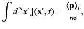 |
(287) |
where
 denotes the expectation value of the momentum
evaluated at time
. Clearly, the probability current is indirectly related to
the particle momentum.
denotes the expectation value of the momentum
evaluated at time
. Clearly, the probability current is indirectly related to
the particle momentum.
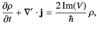
In deriving Equations (284), we have, naturally, assumed that the potential
 is real. Suppose, however, that the potential has an imaginary component.
In this case, Equation (284) generalizes to
is real. Suppose, however, that the potential has an imaginary component.
In this case, Equation (284) generalizes to
 |
(288) |
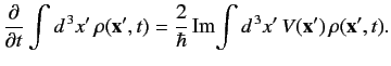
giving
 |
(289) |
Thus, if
 then the total probability of observing the particle
anywhere in space
decreases monotonically with time. Thus, an imaginary potential can be
used to account for the disappearance of a particle. Such a potential
is often employed to model nuclear reactions in which incident particles are
absorbed by nuclei.
then the total probability of observing the particle
anywhere in space
decreases monotonically with time. Thus, an imaginary potential can be
used to account for the disappearance of a particle. Such a potential
is often employed to model nuclear reactions in which incident particles are
absorbed by nuclei.
Next: Exercises
Up: Quantum Dynamics
Previous: Ehrenfest Theorem
Richard Fitzpatrick
2013-04-08