Resonant Layer Response

We saw in Section 5.13 that the relevant linear resonant response regimes in a low-field tokamak fusion reactor are the diffusive-resistive and the viscous-inertial.

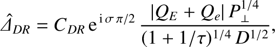
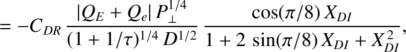
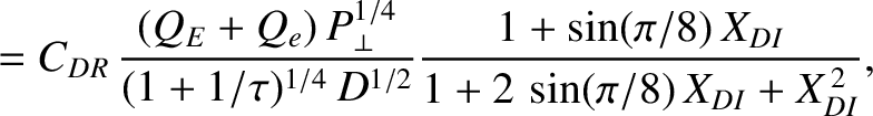
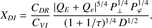
In the diffusive-resistive response regime (see Section 5.9),

$$\skew{6}\hat{\mit\Delta}_{DR} = C_{DR}\,{\rm e}^{\,{\rm i}\,\sigma\,\pi/2}\,\frac{\vert Q_E+Q_e\vert\,P_\perp^{1/4}}{(1+1/\tau)^{1/4}\,D^{1/2}},$$ (7.11)

where $\sigma = {\rm sgn}(Q_E+Q_e)$, and

$$C_{DR} = \frac{2\pi\,{\mit\Gamma}(3/4)}{{\mit\Gamma}(1/4)}.$$ (7.12)

Here, $Q_E = S^{1/3}\,\omega_E\,\tau_H$ and $Q_e= S^{1/3}\,\omega_{\ast\,e}\,\tau_H$, where $\tau _H$ is the hydromagnetic timescale [see Equation (5.43)], $\omega_E$ the E-cross-B frequency [see Equation (5.44)], and $\omega_{\ast\,e}$ the electron diamagnetic frequency [see Equation (5.45)]. All quantities are evaluated at the rational surface. Moreover, $P_\perp = \tau_R/\tau_\perp$ and $D=S^{1/3}\,(1+1/\tau)^{-1/2}\,d_\beta/r_s$, where $\tau_R= S\,\tau_H$ is the resistive diffusion timescale [see Equation (5.49)], $\tau _\perp$ the energy confinement timescale [see Equation (5.52)], $\tau$ the ratio of the electron to the ion pressure gradient [see Equation (4.5)], and $d_\beta$ the ion sound radius [see Equation (4.75)]. In writing expression (7.11), we have made use of the fact that $Q\equiv S^{1/3}\,\omega\,\tau_H=0$ for a static magnetic perturbation.

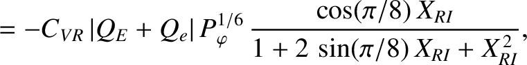
In the viscous-inertial response regime (see Section 5.11),

$$\skew{6}\hat{\mit\Delta}_{VI} =- C_{VI}\,{\rm e}^{-{\rm i}\,\sigma\,\pi/8}\,\vert Q_E+Q_e\vert^{-1/4}\,P_\varphi^{-1/4},$$ (7.13)

where

$$C_{VI} = \frac{\pi}{2}\,\frac{{\mit\Gamma}(1/4)}{{\mit\Gamma}(3/4)}.$$ (7.14)

Here, $P_\varphi= \tau_R/\tau_\varphi$, where $\tau _\varphi$ is the momentum confinement timescale [see Equation (5.50)].

Figure: 7.1 Complex layer matching parameter, $\skew{6}\hat{\mit\Delta}$, calculated from Equations (7.16)–(7.18) for a low-field tokamak fusion reactor. The vertical dashed line corresponds to $Q_E+Q_e=0$.

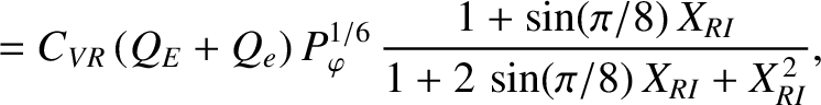
Interpolating between the diffusive-resistive and the viscous-inertial response regimes, we can write

$$\skew{6}\hat{\mit\Delta}= \frac{\skew{6}\hat{\mit\Delta}_{DR}\,\s... ...t\Delta}_{VI}}{ \skew{6}\hat{\mit\Delta}_{DR} + \skew{6}\hat{\mit\Delta}_{VI}}.$$ (7.15)

It follows that in a low-field tokamak fusion reactor,

$${\rm Re}(\skew{6}\hat{\mit\Delta}) = - C_{DR}\,\frac{\vert Q_E+Q_e\vert\,P_\perp^{1/4}}{(1+1/\tau)^{... ...,D^{1/2}}\,\frac{\cos(\pi/8)\,X_{DI}}{1+2\,\sin(\pi/8)\,X_{DI} + X_{DI}^{\,2}},$$ (7.16)

$${\rm Im}(\skew{6}\hat{\mit\Delta}) = C_{DR}\,\frac{(Q_E+Q_e)\,P_\perp^{1/4}}{(1+1/\tau)^{1/4}\,D^{1/2}}\frac{1+\sin(\pi/8)\,X_{DI}}{1+2\,\sin(\pi/8)\,X_{DI} + X_{DI}^{\,2}},$$ (7.17)

where

$$X_{DI} = \frac{C_{DR}}{C_{VI}}\, \frac{\vert Q_E+Q_e\vert^{5/4}\,P_\perp^{1/4}\,P_\varphi^{1/4}}{(1+1/\tau)^{1/4}\,D^{1/2}}.$$ (7.18)

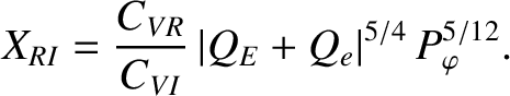
Figure 7.1 shows the real and imaginary components of $\skew{6}\hat{\mit\Delta}$, as functions of the normalized E-cross-B frequency at the rational surface, $Q_E$, calculated from Equations (7.16)–(7.18) for a low-field tokamak fusion reactor. The calculation parameters are $\tau =1$, $Q_{e}=1.00$, $D=3.02$, $P_\varphi=874$, and $P_\perp=287$. (See Table 5.1.) If we compare Figure 7.1 with the exact numerical result shown in Figure 5.5 then we can see that the analytic approximation (7.16)–(7.18) captures most of the salient features of the layer response. In particular, if we had tried to model the layer response just using either the diffusive-resistive or the viscous-inertial response regimes alone then the agreement with the numerical results would have been very poor. The diffusive-resistive response regime predicts that $\skew{6}\hat{\mit\Delta}$ is purely imaginary, and that $\vert{\rm Im}(\skew{6}\hat{\mit\Delta})\vert$ is a monotonically increasing function of $\vert Q_E+Q_e\vert$. On the other hand, the viscous-inertial response regime does not predict a resonance (i.e., a point where $\skew{6}\hat{\mit\Delta}=0$) at $Q_E+Q_e=0$ (i.e., when the electron fluid at the rational surface is stationary). Neither of these prediction are consistent with the data shown in Figure 5.5. Thus, it is clear that, in order to be reasonably accurate, an analytical approximation to the layer response must interpolate between a constant-$\psi$ response regime (in this case, the diffusive-resistive) and a nonconstant-$\psi$ response regime (in this case, the viscous-inertial).

We saw in Section 5.13 that the relevant linear resonant response regimes in a high-field tokamak fusion reactor are the viscous-resistive and the viscous-inertial.

In the viscous-resistive response regime (see Section 5.9),

$$\skew{6}\hat{\mit\Delta}_{VR} = C_{VR}\,{\rm e}^{\,{\rm i}\,\sigma\,\pi/2}\,\vert Q_E+Q_e\vert\,P_\varphi^{1/6},$$ (7.19)

where

$$C_{VR} = \frac{6^{2/3}\,\pi\,{\mit\Gamma}(5/6)}{{\mit\Gamma}(1/6)}.$$ (7.20)

Interpolating between the viscous-resistive and the viscous-inertial response regimes, we can write

$$\skew{6}\hat{\mit\Delta}= \frac{\skew{6}\hat{\mit\Delta}_{VR}\,\s... ...t\Delta}_{VI}}{ \skew{6}\hat{\mit\Delta}_{VR} + \skew{6}\hat{\mit\Delta}_{VI}}.$$ (7.21)

It follows that in a high-field tokamak fusion reactor,

$${\rm Re}(\skew{6}\hat{\mit\Delta}) = - C_{VR}\,\vert Q_E+Q_e\vert\,P_\varphi^{1/6}\,\frac{\cos(\pi/8)\,X_{RI}}{1+2\,\sin(\pi/8)\,X_{RI} + X_{RI}^{\,2}},$$ (7.22)

$${\rm Im}(\skew{6}\hat{\mit\Delta}) = C_{VR}\,(Q_E+Q_e)\,P_\varphi^{1/6}\,\frac{1+\sin(\pi/8)\,X_{RI}}{1+2\,\sin(\pi/8)\,X_{RI} + X_{RI}^{\,2}},$$ (7.23)

where

$$X_{RI} = \frac{C_{VR}}{C_{VI}}\, \vert Q_E+Q_e\vert^{5/4}\,P_\varphi^{5/12}.$$ (7.24)

Figure: 7.2 Complex layer matching parameter, $\skew{6}\hat{\mit\Delta}$, calculated from Equations (7.22)–(7.24) for a high-field tokamak fusion reactor. The vertical dashed line corresponds to $Q_E+Q_e=0$.

Figure 7.2 shows the real and imaginary components of $\skew{6}\hat{\mit\Delta}$, as functions of the normalized E-cross-B frequency at the rational surface, $Q_E$, calculated from Equations (7.22)–(7.24) for a high-field tokamak fusion reactor. The calculation parameters are $Q_{e}=0.75$, and $P_\varphi=874$. (See Table 5.1.) As before, if we compare Figure 7.2 with the exact numerical result shown in Figure 5.6 then we can see that the analytic approximation (7.22)–(7.24) captures most of the salient features of the layer response.