Next: Error-Field Penetration Up: Error-Field Penetration in Tokamak Previous: Resonant Layer Response Contents
 , that develops in response to the electromagnetic
torque exerted at the surface by the error-field (see Section 3.13), is mirrored by an equal shift in the ion fluid rotation frequency (as well as in the electron fluid rotation frequency). This is the
essence of the no-slip constraint, (3.185), which follows from Equations (2.321) and (2.322)
because the torque modifies the E-cross-B velocity at the rational surface, but does not affect the diamagnetic velocities.
, that develops in response to the electromagnetic
torque exerted at the surface by the error-field (see Section 3.13), is mirrored by an equal shift in the ion fluid rotation frequency (as well as in the electron fluid rotation frequency). This is the
essence of the no-slip constraint, (3.185), which follows from Equations (2.321) and (2.322)
because the torque modifies the E-cross-B velocity at the rational surface, but does not affect the diamagnetic velocities.
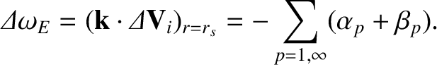
Equations (3.190) and (3.191) yield
where we have set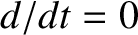 (because the error-field is static). Here,
 |
![$\displaystyle = \tau_{\theta\,i}(r_s) = \left[\frac{\tau_i}{\sqrt{2}\,\mu_{i\,11}\,f_t}\left(\frac{\epsilon}{q}\right)^2\right]_{r=r_s},$](img2547.png) |
(7.28) |
 |
 |
(7.29) |
 |
 |
(7.30) |
 |
 |
(7.31) |
 ,
,
 , and
, and
 .
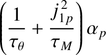
Furthermore, the dimensionless neoclassical viscosity parameter
.
Furthermore, the dimensionless neoclassical viscosity parameter
 is
defined in Equation (2.204),
is
defined in Equation (2.204),
 is the ion poloidal flow-damping timescale,
  the fraction of trapped particles [see Equation (2.202)],
  the ion-ion collision time [see Equation (2.21)],
  the safety-factor profile (see Section 3.2), and
 the magnetic shear at the
rational surface [see Equation (5.28)]. Moreover,
the magnetic shear at the
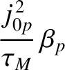
rational surface [see Equation (5.28)]. Moreover,  denotes a Bessel function, whereas
  and
and  denote the
  th zeros of the
  and
and  Bessel functions, respectively.
![\includegraphics[width=1.\textwidth]{Chapter07/Figure7_3.eps}](img2561.png)
|
Let
 |
(7.32) |
 is the E-cross-B frequency at the rational surface in the absence of the error-field.
It is helpful to define
is the E-cross-B frequency at the rational surface in the absence of the error-field.
It is helpful to define
 .
Equations (7.25)–(7.27) can be combined to give
where
.
Equations (7.25)–(7.27) can be combined to give
where  .
Here, use has been made of the results [7]
.
Here, use has been made of the results [7]
Equations (7.9), (7.10), and (7.33) yield the torque balance equation [4,6]
where |
 |
(7.37) |
 |
 |
(7.38) |
 |
 |
(7.39) |
 |
![$\displaystyle =\frac{1}{2\,\epsilon_s\,s_s}\left[\left(\frac{q_s}{\epsilon_s}\r...
...c{a}{r_s}\right)\right]^{1/2}\left(\frac{S}{P_\varphi}\right)^{1/2}\tilde{I}_c.$](img2577.png) |
(7.40) |
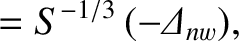
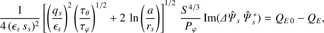
Equation (7.36) can be rearranged to give
where![$\displaystyle F(Q_E) = (Q_{E\,0} -Q_E) \,\frac{[\zeta+\skew{6}\hat{\mit\Delta}_r(Q_E)]^2
+ [\skew{6}\hat{\mit\Delta}_i(Q_E)]^2}{\skew{6}\hat{\mit\Delta}_i(Q_E)}.$](img2579.png) |
(7.42) |
![\includegraphics[width=1.\textwidth]{Chapter07/Figure7_4.eps}](img2581.png)
|
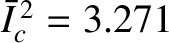
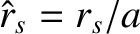
Figure 7.3 shows the torque balance function,  , calculated for a low-field tokamak fusion reactor with
 .
The parameters used in the calculation are
.
The parameters used in the calculation are  ,
,
 ,
,  ,
,
 , and
, and
 , as well as
 ,
,  , and
, and
 . (See Tables 5.1 and 6.1.) Note that
 and
and
 are specified in Equations (7.16) and
(7.17), respectively. The parameter
are specified in Equations (7.16) and
(7.17), respectively. The parameter  takes the value
 . As indicated in the figure,
when
. As indicated in the figure,
when
 there are three possible values of the normalized E-cross-B frequency at the rational
surface,
there are three possible values of the normalized E-cross-B frequency at the rational
surface,  , that satisfy Equation (7.41). However, as is
easily demonstrated, the
middle solution is dynamically unstable [4]. We thus conclude that there are two dynamically stable
branches of solutions to the torque balance equation, (7.36). On the high-slip branch (i.e., the rightmost solution in the figure), the electron
fluid at the rational surface rotates with respect to the error-field, generating a shielding current that suppresses
driven magnetic reconnection. On the low-slip branch (i.e., the leftmost solution in the figure), the
electron fluid rotation at the rational surface is arrested, there is no shielding current, and driven magnetic
reconnection proceeds unhindered.
, that satisfy Equation (7.41). However, as is
easily demonstrated, the
middle solution is dynamically unstable [4]. We thus conclude that there are two dynamically stable
branches of solutions to the torque balance equation, (7.36). On the high-slip branch (i.e., the rightmost solution in the figure), the electron
fluid at the rational surface rotates with respect to the error-field, generating a shielding current that suppresses
driven magnetic reconnection. On the low-slip branch (i.e., the leftmost solution in the figure), the
electron fluid rotation at the rational surface is arrested, there is no shielding current, and driven magnetic
reconnection proceeds unhindered.
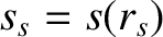
Figure 7.4 shows the torque balance function, , calculated for a high-field tokamak fusion reactor with
.
The parameters used in the calculation are
 , and
, as well as
, and
, as well as
 , , and
. (See Tables 5.1 and 6.1.) Note that
and
are specified in Equations (7.22) and
(7.23), respectively. The parameter takes the value
, , and
. (See Tables 5.1 and 6.1.) Note that
and
are specified in Equations (7.22) and
(7.23), respectively. The parameter takes the value
 .
As indicated in the figure, when
.
As indicated in the figure, when
 attains the critical value
  , the high-slip and the dynamically
unstable solutions of the torque balance equation merge together and annihilate one another. For
, the high-slip and the dynamically
unstable solutions of the torque balance equation merge together and annihilate one another. For
 ,
only the low-slip solution branch exists. Thus, if the system is initially on the high-slip solution branch, and the
error-field amplitude is raised such that
exceeds the critical value 3.271, then there is a bifurcation
from the high-slip to the low-slip solution branch. This bifurcation is associated with the sudden arrest of the
electron fluid rotation at the rational surface, the collapse of the shielding current, and the onset of driven magnetic
reconnection [4,6]. Of course, the bifurcation corresponds to the error-field penetration phenomenon discussed in
Section 7.1.
,
only the low-slip solution branch exists. Thus, if the system is initially on the high-slip solution branch, and the
error-field amplitude is raised such that
exceeds the critical value 3.271, then there is a bifurcation
from the high-slip to the low-slip solution branch. This bifurcation is associated with the sudden arrest of the
electron fluid rotation at the rational surface, the collapse of the shielding current, and the onset of driven magnetic
reconnection [4,6]. Of course, the bifurcation corresponds to the error-field penetration phenomenon discussed in
Section 7.1.
![\includegraphics[width=1.\textwidth]{Chapter07/Figure7_5.eps}](img2593.png)
|
![$\displaystyle = \frac{m^{2}\,[J_1(j_{1p}\,\hat{r}_s)]^{\,2}}{\tau_A^{\,2}\,\eps...
...,{\rm Im}({\mit\Delta\skew{3}\hat{\Psi}}_s\,\skew{3}\hat{\mit\Psi}_s^{\,\ast}),$](img2543.png)
![$\displaystyle = \frac{n^{2}\,[J_0(j_{0p}\,\hat{r}_s)]^{\,2}}{\tau_A^{\,2}\,[J_1...
...
{\rm Im}({\mit\Delta\skew{3}\hat{\Psi}}_s\,\skew{3}\hat{\mit\Psi}_s^{\,\ast}),$](img2545.png)
![$\displaystyle \lim_{\epsilon\rightarrow 0}\sum_{p=1,\infty} \frac{\sqrt{\epsilon}\,[J_1(j_{1p}\,x)]^{2}}{[J_2(j_{1p})]^2\,(1+\epsilon\,j_{1p}^{\,2})}$](img2567.png)

![$\displaystyle \sum_{p=1,\infty} \frac{[J_0(j_{0p}\,x)]^2}{[J_1(j_{0p})]^2\,j_{0p}^{\,2}} =\frac{1}{2}\,\ln\left(\frac{1}{x}\right).$](img2569.png)
![$\displaystyle \frac{\skew{6}\hat{\mit\Delta}_i(Q_E)\,\bar{I}_c^{\,2}}{[\zeta+\s...
...hat{\mit\Delta}_r(Q_E)]^2
+ [\skew{6}\hat{\mit\Delta}_i(Q_E)]^2}=Q_{E\,0} -Q_E,$](img2570.png)