Ionospheric Ray Tracing

Suppose that we possess a radio antenna that is capable of launching radio waves of constant frequency $\omega$ into the ionosphere at an angle to the vertical. Let us consider the paths traced out by these waves in the $x$ -$z$ plane. For the sake of simplicity, we shall assume that the waves are horizontally polarized, so that the electric field vector always lies parallel to the $y$ -axis. The signal emitted by the antenna (located at $z=0$ ) can be represented as

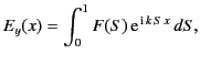$$E_y(x) = \int_{0}^{1} F(S) \,{\rm e}^{\,{\rm i}\,k \,S\,x}\,dS,$$ (1138)

where $k=\omega/c$ . Here, the ${\rm e}^{-{\rm i}\,\omega\, t}$ time dependence of the signal has been neglected for the sake of clarity. Suppose that the signal emitted by the antenna is mostly concentrated in a direction making an angle $\theta_I$ with the vertical. It follows that $F(S)$ possesses a narrow maximum around $S=S_0$ , where $S_0= \sin\theta_I$ .

If Equation (1140) represents the signal at ground level then the signal at height $z$ in the ionosphere is easily obtained by making use of the WKB solution for horizontally polarized waves described in Section 8.9. We obtain

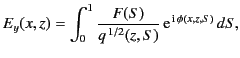$$E_y(x,z) =\int_{0}^1 \frac{F(S)}{q^{\,1/2}(z,S)} \,{\rm e}^{\,{\rm i}\,\phi (x,z,S)}\,dS,$$ (1139)

where

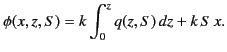$$\phi(x,z,S) = k\int_0^z q(z,S)\,dz + k\,S\,x.$$ (1140)

Equation (1141) is essentially a contour integral in $S$ -space. The quantity $F/q^{\,1/2}$ is a relatively slowly varying function of $S$ , whereas the phase $\phi$ is a large and rapidly varying function of $S$ . As described in Section 7.12, the rapid oscillations of $\exp(\,{\rm i}\,\phi)$ over most of the path of integration ensure that the integrand averages almost to zero. In fact, only those points on the path of integration where the phase is stationary (i.e., where $\partial\phi/\partial S = 0$ ) make a significant contribution to the integral. It follows that the left-hand side of Equation (1141) averages to a very small value, except for those special values of $x$ and $z$ at which one of the points of stationary phase in $S$ -space coincides with the peak of $F(S)$ . The locus of these special values of $x$ and $z$ can clearly be regarded as the trajectory of the radio signal emitted by the antenna as it passes through the ionosphere. Thus, the signal trajectory is specified by

$$\left(\frac{\partial\phi}{\partial S}\right)_{S=S_0} = 0,$$ (1141)

which yields

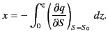$$x = - \int_0^z \left(\frac{\partial q}{\partial S}\right)_{S=S_0}\,dz.$$ (1142)

We can think of this equation as tracing the path of a ray of radio frequency radiation, emitted by the antenna at an angle $\theta_I$ to the vertical (where $S_0= \sin\theta_I$ ), as it propagates through the ionosphere.

Now

$$q^{\,2} = n^{\,2} - S^{\,2},$$ (1143)

so the ray tracing equation becomes

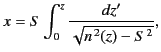$$x = S \int_0^z \frac{dz'}{\sqrt{n^{\,2}(z)-S^{\,2}}},$$ (1144)

where $S$ is the sine of the initial (i.e., at the antenna) angle of incidence of the ray with respect to the vertical axis. Of course, Equation (1146) only holds for upgoing rays. For downgoing rays, a simple variant of the previous analysis using the downgoing WKB solutions yields

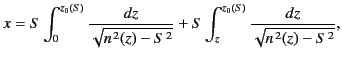$$x = S\int_0^{z_0(S)} \frac{dz}{\sqrt{n^{\,2}(z)-S^{\,2}} } + S\int_z^{z_0(S)} \frac{dz}{\sqrt{n^{\,2}(z)-S^{\,2}}},$$ (1145)

where $n(z_0) = S$ . Thus, the ray ascends into the ionosphere after being launched from the antenna, reaches a maximum height $z_0$ above the surface of the Earth, and then starts to descend. The ray eventually intersects the Earth's surface again a horizontal distance

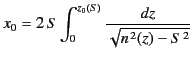$$x_0 = 2 \,S\int_0^{z_0(S)} \frac{dz}{\sqrt{n^{\,2}(z)-S^{\,2}} }$$ (1146)

away from the antenna.

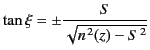
The angle $\xi$ which the ray makes with the vertical is given by $\tan\xi = dx/dz$ . It follows from Equations (1146) and (1147) that

$$\tan\xi =\pm \frac{S}{\sqrt{n^{\,2}(z)-S^{\,2}}}$$ (1147)

where the upper and lower signs correspond to the upgoing and downgoing parts of the ray trajectory, respectively. Note that $\xi=\pi/2$ at the reflection point, where $n=S$ . Thus, the ray is horizontal at the reflection point.

Let us investigate the reflection process in more detail. In particular, we wish to demonstrate that radio waves are reflected at the $q=0$ surface, rather than being absorbed. We would also like to understand the origin of the $-\pi/2$ phase shift of radio waves at reflection which is evident in Equation (1107). In order to achieve these goals, we shall need to review the mathematics of asymptotic series.