Next: Ionospheric Pulse Propagation
Up: Wave Propagation in Inhomogeneous
Previous: Reflection Coefficient
Extension to Oblique Incidence
We have discussed the WKB solution for radio waves propagating vertically
through an ionosphere whose refractive index varies slowly with height. Let us now
generalize this solution to take into account radio waves that propagate at an
angle to the vertical axis.
The refractive index of the ionosphere is assumed to vary continuously with height,  .
However, let us, for the sake of clarity, imagine that the ionosphere is replaced by
a number of thin, discrete, homogeneous, horizontal strata. A
continuous ionosphere corresponds to the limit in which the
strata become innumerable and infinitely thin. Suppose that a plane wave is incident from below on the ionosphere. Let the wave normal lie in the
.
However, let us, for the sake of clarity, imagine that the ionosphere is replaced by
a number of thin, discrete, homogeneous, horizontal strata. A
continuous ionosphere corresponds to the limit in which the
strata become innumerable and infinitely thin. Suppose that a plane wave is incident from below on the ionosphere. Let the wave normal lie in the
 -
plane, and subtend an angle
-
plane, and subtend an angle  with
the vertical axis. At the lower boundary of the first stratum, the wave is partially
reflected and partially transmitted. The transmitted wave is then partially reflected
and partially transmitted at the lower boundary of the second stratum, and so on.
However, in the limit of many strata, in which the difference in refractive indices
between
neighboring strata is very small, the amount of reflection at the boundaries (which is
proportional to the square of this difference)
becomes negligible. In the
with
the vertical axis. At the lower boundary of the first stratum, the wave is partially
reflected and partially transmitted. The transmitted wave is then partially reflected
and partially transmitted at the lower boundary of the second stratum, and so on.
However, in the limit of many strata, in which the difference in refractive indices
between
neighboring strata is very small, the amount of reflection at the boundaries (which is
proportional to the square of this difference)
becomes negligible. In the  th stratum, let
  be the refractive
index, and let
be the refractive
index, and let  be the angle subtended between the wave normal and the vertical
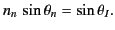
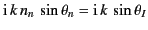
axis. According to Snell's law,
be the angle subtended between the wave normal and the vertical
axis. According to Snell's law,
 |
(1088) |
Below the ionosphere  , and so
 |
(1089) |
For an electromagnetic wave in the
th stratum, a general
field quantity depends on
and
via
factors of the form
![$\displaystyle A\,{\rm\exp}\left[\,{\rm i}\,k \,n_n(\pm z\cos\theta_n + x\sin\theta_n)\right],$](img2290.png) |
(1090) |
where  is a constant.
The
is a constant.
The  signs denote upgoing and downgoing waves, respectively.
When the operator
signs denote upgoing and downgoing waves, respectively.
When the operator
 acts on the previous expression, it is equivalent to
multiplication by
acts on the previous expression, it is equivalent to
multiplication by
 ,
which is independent of
and
. It is convenient to use the
notation
,
which is independent of
and
. It is convenient to use the
notation
 . Hence, we may write symbolically
These results are true no matter how thin the strata are, so they must also
hold for a continuous ionosphere. Note that, according to
Snell's law, if the wave normal is initially parallel to the
-
plane then it will remain parallel to this plane as the wave
propagates through the ionosphere.
Equations (1058)-1061) and (1093)-(1094) can be combined to give
and
As before, Maxwell's equations can be split into two independent groups, corresponding
to two different polarizations of radio waves propagating through the ionosphere.
For the first group of equations, the electric field is always parallel
to the  -axis. The corresponding waves are, therefore, said to be horizontally
polarized. For the second group of equations, the electric field always
lies in the
-
plane. The corresponding waves are, therefore, said
to be vertically polarized. (However, the term ``vertically
polarized'' does not necessarily imply that the electric field is parallel
to the vertical axis.) Note that the equations governing horizontally
polarized waves are not isomorphic to those governing vertically
polarized waves. Consequently, both types of waves must be dealt with separately.
-axis. The corresponding waves are, therefore, said to be horizontally
polarized. For the second group of equations, the electric field always
lies in the
-
plane. The corresponding waves are, therefore, said
to be vertically polarized. (However, the term ``vertically
polarized'' does not necessarily imply that the electric field is parallel
to the vertical axis.) Note that the equations governing horizontally
polarized waves are not isomorphic to those governing vertically
polarized waves. Consequently, both types of waves must be dealt with separately.
For the case of horizontally polarized waves, Equations (1096) and (1097)
yield
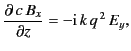 |
(1099) |
where
 |
(1100) |
The previous equation can be combined with Equation (1095) to give
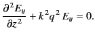 |
(1101) |
Equations (1101) and (1103) have exactly the same form as Equations (1064)
and (1067), except that  is replaced by
  . Hence, the analysis of
Section 783 can be reused to find the appropriate WKB solution, which take the
form
. Hence, the analysis of
Section 783 can be reused to find the appropriate WKB solution, which take the
form
where
is a constant. Of course, both expressions should also contain a
multiplicative
factor
 , but this is usually
omitted for the sake of clarity. By analogy with Equation (1079), the
previous WKB solution is valid as long as
, but this is usually
omitted for the sake of clarity. By analogy with Equation (1079), the
previous WKB solution is valid as long as
 |
(1104) |
This inequality clearly fails in the vicinity of  , no matter how
slowly
, no matter how
slowly  varies with
. Hence,
, which is equivalent to
varies with
. Hence,
, which is equivalent to
 , specifies the
height at which reflection takes place. By analogy with
Equation (1089), the reflection coefficient at ground level (
, specifies the
height at which reflection takes place. By analogy with
Equation (1089), the reflection coefficient at ground level ( ) is
given by
) is
given by
 |
(1105) |
where  is the height at which
.
is the height at which
.
For the case of vertical polarization, Equations (1098) and (1100) yield
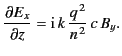 |
(1106) |
This equation can be combined with Equation (1099) to give
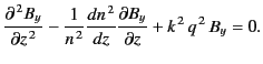 |
(1107) |
Clearly, the differential equation that governs the propagation
of vertically polarized waves is
considerably more complicated than the corresponding equation
for horizontally polarized waves.
The WKB solution for vertically polarized waves is obtained by substituting the
wave-like solution
 |
(1108) |
where
is a constant, and  is the generalized phase,
into Equation (1109). The differential equation thereby obtained for the phase
is
is the generalized phase,
into Equation (1109). The differential equation thereby obtained for the phase
is
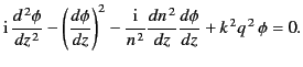 |
(1109) |
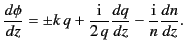
Because the refractive index is assumed to be slowly varying, the first and third term in the previous
equation are small, and so, to a first approximation,
These expressions can be substituted into the first and third terms of
Equation (1111) to give the second approximation,
![$\displaystyle \frac{d\phi}{dz}=\pm \left[k^{\,2} q^{\,2} \pm {\rm i}\,k\left( \frac{dq}{dz} - \frac{2\,q}{n} \frac{dn}{dz}\right)\right]^{1/2}.$](img2325.png) |
(1112) |
The final two terms on the right-hand side of the previous equation are
small, so expansion of the right-hand side by means of the binomial theorem
yields
 |
(1113) |
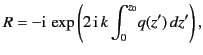
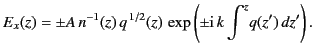
This expression can be integrated, and the result substituted into Equation (1110),
to give the WKB solution
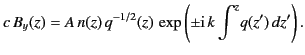 |
(1114) |
The corresponding WKB solution for  is obtained from Equation (1108):
 |
(1115) |
Here, any terms involving derivatives of
and
have been neglected.
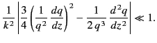
Substituting Equation (1116) into the differential equation (1109),
and demanding that the remainder be small compared to the original terms in the
equation, yields the following condition for
the validity of the previous WKB solution:
![$\displaystyle \frac{1}{k^{\,2}}\left\vert \frac{3}{4}\left(\frac{1}{q^{\,2}} \f...
... z^{\,2}} -2 \left(\frac{1}{n} \frac{d n}{dz}\right)^2\right]\right\vert \ll 1.$](img2329.png) |
(1116) |
This criterion fails close to
, no matter how slowly
and
vary with
. Hence,
gives the height
at which reflection takes place. The condition also fails close to  ,
which does not correspond to the reflection level. If, as is usually the case, the electron
density in the ionosphere increases monotonically with height then the level
at which
lies above the reflection level (where
). If the
two levels are well separated then the reflection process is unaffected by the
failure of the previous inequality at the level
, and the reflection coefficient
is given by Equation (1107), just as is the case for the
horizontal polarization. If, however,
the level
lies close to the level
then the reflection coefficient
may be affected, and a more accurate treatment of the differential
equation (1109) is required in order
to obtain the true value of the reflection coefficient.
,
which does not correspond to the reflection level. If, as is usually the case, the electron
density in the ionosphere increases monotonically with height then the level
at which
lies above the reflection level (where
). If the
two levels are well separated then the reflection process is unaffected by the
failure of the previous inequality at the level
, and the reflection coefficient
is given by Equation (1107), just as is the case for the
horizontal polarization. If, however,
the level
lies close to the level
then the reflection coefficient
may be affected, and a more accurate treatment of the differential
equation (1109) is required in order
to obtain the true value of the reflection coefficient.
Next: Ionospheric Pulse Propagation
Up: Wave Propagation in Inhomogeneous
Previous: Reflection Coefficient
Richard Fitzpatrick
2014-06-27