


Next: WKB Approximation
Up: Wave Propagation in Inhomogeneous
Previous: Reflection by Conducting Surfaces
Let us investigate the propagation of an electromagnetic wave though a spatially
non-uniform dielectric medium.
As a specific example, consider the
propagation of radio waves through the Earth's ionosphere. The refractive
index of the ionosphere can be written [see Equation (801)]
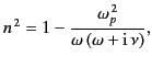 |
(1054) |
where  is a real positive constant that parameterizes the damping of electron
motion
(in fact,
is the collision frequency of free electrons with other
particles in the ionosphere), and
is a real positive constant that parameterizes the damping of electron
motion
(in fact,
is the collision frequency of free electrons with other
particles in the ionosphere), and
 |
(1055) |
is the plasma frequency. In the previous formula,  is the density of
free electrons in the ionosphere, and
is the density of
free electrons in the ionosphere, and  is the electron mass. We shall
assume that the ionosphere is horizontally stratified, so that
is the electron mass. We shall
assume that the ionosphere is horizontally stratified, so that  ,
where the coordinate
,
where the coordinate  measures height above the Earth's surface (the curvature of the Earth's surface is neglected in the following analysis). The ionosphere
actually consists of two main layers; the E-layer, and the F-layer. We shall
concentrate on the lower E-layer, which lies about 100 km above the surface
of the Earth, and is about 50 km thick. The typical day-time number density
of free electrons in the E-layer is
measures height above the Earth's surface (the curvature of the Earth's surface is neglected in the following analysis). The ionosphere
actually consists of two main layers; the E-layer, and the F-layer. We shall
concentrate on the lower E-layer, which lies about 100 km above the surface
of the Earth, and is about 50 km thick. The typical day-time number density
of free electrons in the E-layer is
 .
At night-time, the density of free electrons falls to about half this number.
The typical day-time plasma frequency of the E-layer is, therefore, about 5 MHz.
The typical collision frequency of free electrons in the E-layer
is about 0.05 MHz.
According to simplistic theory, any radio wave whose frequency lies below the
day-time plasma frequency,
5 MHz, (i.e., any wave whose wavelength exceeds about 60 m) is reflected
by the ionosphere during the day. Let us investigate in more detail how this
process takes place. Note, incidentally, that
.
At night-time, the density of free electrons falls to about half this number.
The typical day-time plasma frequency of the E-layer is, therefore, about 5 MHz.
The typical collision frequency of free electrons in the E-layer
is about 0.05 MHz.
According to simplistic theory, any radio wave whose frequency lies below the
day-time plasma frequency,
5 MHz, (i.e., any wave whose wavelength exceeds about 60 m) is reflected
by the ionosphere during the day. Let us investigate in more detail how this
process takes place. Note, incidentally, that
 for mega-Hertz
frequency radio waves, so it follows from Equation (1056) that
for mega-Hertz
frequency radio waves, so it follows from Equation (1056) that
 is predominately real (i.e., under
normal circumstances, electron collisions can be neglected).
is predominately real (i.e., under
normal circumstances, electron collisions can be neglected).
The problem of radio wave propagation through the ionosphere was
of great practical importance during the first half of the 20th century, because,
during that period, long-wave radio waves were the principal means of military communication.
Nowadays, the military have far more reliable methods of communication. Nevertheless,
this subject area is still worth studying, because the principal tool used
to deal with the problem of wave propagation through a non-uniform medium--the
so-called WKB approximation--is of great theoretical importance. In particular,
the WKB approximation is very widely used in quantum mechanics (in fact, there
is a great similarity between the problem of wave propagation through
a non-uniform medium, and the problem of solving Schrödinger's equation
in the presence of a non-uniform potential).
Maxwell's equations for a wave propagating through a non-uniform,
unmagnetized, dielectric medium are
where  is the non-uniform refractive index of the medium. It is
assumed that all field quantities vary in time like
is the non-uniform refractive index of the medium. It is
assumed that all field quantities vary in time like
 , where
 . Note that, in the following,
  is the
wavenumber in free space, rather than the wavenumber in the dielectric medium.
is the
wavenumber in free space, rather than the wavenumber in the dielectric medium.
Next: WKB Approximation
Up: Wave Propagation in Inhomogeneous
Previous: Reflection by Conducting Surfaces
Richard Fitzpatrick
2014-06-27