


Next: High Frequency Limit
Up: Wave Propagation in Uniform
Previous: Anomalous Dispersion and Resonant
Wave Propagation in Conducting Media
In the limit
 , there is a significant difference in
the response of a dielectric medium to an electromagnetic wave, depending on whether the lowest resonant
frequency is zero or non-zero. For insulators, the lowest
resonant frequency is different from zero. In this case, the low frequency
refractive index is predominately real, and is also greater than unity.
In a conducting medium, on the other hand, some fraction,
, there is a significant difference in
the response of a dielectric medium to an electromagnetic wave, depending on whether the lowest resonant
frequency is zero or non-zero. For insulators, the lowest
resonant frequency is different from zero. In this case, the low frequency
refractive index is predominately real, and is also greater than unity.
In a conducting medium, on the other hand, some fraction,  , of the electrons are ``free,'' in
the sense of having
, of the electrons are ``free,'' in
the sense of having
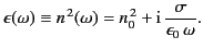
 . In this situation, the low frequency dielectric
constant takes the form
. In this situation, the low frequency dielectric
constant takes the form
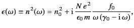 |
(800) |
where  is the contribution to
the refractive index from all of the other resonances, and
is the contribution to
the refractive index from all of the other resonances, and
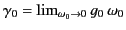 . Consider the Ampère-Maxwell equation,
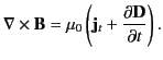 |
(801) |
Here,  is the true current: that is, the current carried by free, as opposed to bound, charges.
Let us assume that the medium in question obeys Ohm's law,
is the true current: that is, the current carried by free, as opposed to bound, charges.
Let us assume that the medium in question obeys Ohm's law,
 , and has a ``normal''
dielectric constant
, and has a ``normal''
dielectric constant  . Here,
  is the conductivity.
Assuming an
is the conductivity.
Assuming an
 time dependence of all field quantities,
the previous equation yields
time dependence of all field quantities,
the previous equation yields
 |
(802) |
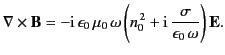
Suppose, however, that we do not explicitly use Ohm's law but, instead, attribute
all of the properties of the medium to the dielectric constant. In this case,
the effective dielectric constant of the medium is equivalent to the term in
round brackets on the right-hand side of the previous equation: that is,
 |
(803) |
A comparison of this term with Equation (801) yields the following expression for
the conductivity,
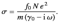 |
(804) |
Thus, at low frequencies, conductors possess predominately real conductivities
(i.e., the current remains in phase with the electric field). However, at
higher frequencies, the conductivity becomes complex. At such frequencies,
there is little meaningful distinction between a conductor and an insulator, because
the ``conductivity'' contribution to
 appears as a resonant
amplitude, just like the other contributions. For a good conductor, such as copper,
the conductivity remains predominately real for all frequencies up to, and including,
those in the microwave region of the electromagnetic spectrum.
appears as a resonant
amplitude, just like the other contributions. For a good conductor, such as copper,
the conductivity remains predominately real for all frequencies up to, and including,
those in the microwave region of the electromagnetic spectrum.
The conventional way in which to represent the complex refractive index of
a conducting medium (in the low frequency limit) is to write it in terms
of a real ``normal'' dielectric constant,
 , and a real
conductivity,
. Thus, from Equation (804),
, and a real
conductivity,
. Thus, from Equation (804),
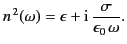 |
(805) |
For a poor conductor (i.e.,
 ), we find that
 |
(806) |
In this limit,
 , and the attenuation
of the wave, which is governed by
, and the attenuation
of the wave, which is governed by
 [see Equation (776)], is
independent of the frequency. Thus, for a poor conductor, the wave acts like a wave propagating through a conventional dielectric
of dielectric constant
[see Equation (776)], is
independent of the frequency. Thus, for a poor conductor, the wave acts like a wave propagating through a conventional dielectric
of dielectric constant  , except that it attenuates gradually
over a distance of very many wavelengths.
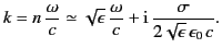
For a good conductor
(i.e.,
, except that it attenuates gradually
over a distance of very many wavelengths.
For a good conductor
(i.e.,
 ), we obtain
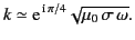 |
(807) |
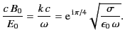
It follows from Equation (772) that
 |
(808) |
Thus, the phase of the magnetic field lags that of the electric field by
 radians. Moreover, the magnitude of
  is much larger than that of
  (because
 ). It follows that the
wave energy is almost entirely magnetic in nature. Clearly, an electromagnetic wave propagating through a good conductor has markedly different properties
to a wave propagating through a conventional
dielectric. For a wave propagating
in the
). It follows that the
wave energy is almost entirely magnetic in nature. Clearly, an electromagnetic wave propagating through a good conductor has markedly different properties
to a wave propagating through a conventional
dielectric. For a wave propagating
in the  -direction, the amplitudes of the electric and magnetic fields
attenuate like
-direction, the amplitudes of the electric and magnetic fields
attenuate like
 , where
 |
(809) |
is termed the skin depth. It is apparent that an electromagnetic
wave incident on a conducting medium will not penetrate more than a few skin depths
into that medium.
Next: High Frequency Limit
Up: Wave Propagation in Uniform
Previous: Anomalous Dispersion and Resonant
Richard Fitzpatrick
2014-06-27