Introduction

As is easily demonstrated, the fields associated with an electromagnetic wave propagating through a uniform dielectric medium of dielectric constant $\epsilon$ satisfy

$$\left(\frac{\epsilon}{c^{\,2}}\frac{\partial^{\,2}}{\partial t^{\,2}}-\nabla^{\,2}\right) {\bf E} = {\bf0},$$ (767)

and

$$\nabla\times{\bf E} = -\frac{\partial{\bf B}}{\partial t}.$$ (768)

The plane wave solutions to these equations are well known:

$${\bf E} = {\bf E}_0\, \exp\left[\,{\rm i}\,({\bf k}\cdot{\bf r}-\omega \,t)\right],$$ (769)

$${\bf B} ={\bf B}_0 \,\exp\left[\,{\rm i}\,({\bf k}\cdot{\bf r}-\omega \,t)\right],$$ (770)

where ${\bf E}_0$ and ${\bf B}_0$ are constant vectors,

$$\frac{\omega^{\,2}}{k^{\,2}} = \frac{c^{\,2}}{\epsilon},$$ (771)

and

$${\bf B}_0 = \frac{{\bf k}\times{\bf E}_0}{\omega}.$$ (772)

The phase velocity of the wave is given by

$$v = \frac{\omega}{k} = \frac{c}{n},$$ (773)

where

$$n = \sqrt{\epsilon}$$ (774)

is the medium's refractive index. Thus, in a conventional dielectric medium (i.e., $\epsilon$ real and greater than unity), an electromagnetic wave propagates with a phase velocity that is slower than the velocity of light in vacuum.

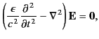
In some dielectric media, the dielectric constant, $\epsilon$ , is complex. According to Equation (772), this leads to a complex wavevector, ${\bf k}$ (assuming that the angular frequency is real). Thus, for a wave propagating in the $x$ -direction, we obtain

$${\bf E} = {\bf E}_0\,\exp(\,{\rm i}\,[{\rm Re}(k)\, x -\omega \,t]) \exp[-{\rm Im}(k) \,x].$$ (775)

In other words, a complex dielectric constant leads to the attenuation (or amplification) of the wave, as it propagates through the medium.

Up to now, we have tacitly assumed that $\epsilon$ is the same for waves of all frequencies. In practice, $\epsilon$ varies (in some cases, strongly) with the wave frequency. Consequently, waves of different frequencies propagate through a dielectric medium at different phase velocities, leading to the dispersion of wave pulses. Moreover, there may exist frequency bands in which the waves are attenuated (i.e., absorbed). All of this makes the problem of determining the behavior of a wave pulse as it propagates through a dielectric medium a far from straightforward task. Of course, the solution to this problem for a wave pulse traveling through a vacuum is fairly trivial: that is, the pulse propagates at the velocity $c$ without changing shape. What is the equivalent result for the case of a dielectric medium? This is a significant question, because most of our information regarding the universe is obtained from the study of electromagnetic waves emitted by distant objects. All of these waves have to propagate through dispersive media (e.g., the interstellar medium, the ionosphere, the atmosphere) before reaching us. It is, therefore, vitally important that we understand which aspects of these wave signals are predominantly determined by the wave sources, and which are strongly modified by the dispersive media through which the signals have propagated in order to reach us.