


Next: Ionospheric Ray Tracing
Up: Wave Propagation in Inhomogeneous
Previous: Ionospheric Pulse Propagation
The equivalent height of the ionosphere can be measured
in a fairly straightforward manner,
by timing how long it takes a radio pulse fired vertically
upwards to return to ground level again.
We can, therefore, determine
the function  experimentally by performing this procedure
many times with pulses of different central frequencies.
But, is it possible to
use this information to determine the number density of free electrons in the
ionosphere as a function of height? In mathematical terms, the problem
is as follows. Does a knowledge of the function
experimentally by performing this procedure
many times with pulses of different central frequencies.
But, is it possible to
use this information to determine the number density of free electrons in the
ionosphere as a function of height? In mathematical terms, the problem
is as follows. Does a knowledge of the function
![$\displaystyle h(\omega) = \int_0^{z_0(\omega)} \frac{\omega}{[\omega^{\,2}-\omega_p^{\,2}(z)]^{1/2}} \,dz,$](img2356.png) |
(1131) |
where
 , necessarily imply a knowledge
of the function
, necessarily imply a knowledge
of the function
 ?
Recall that
?
Recall that
 .
.
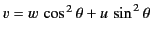
Let
 and
and
 . Equation (1133)
then becomes
. Equation (1133)
then becomes
![$\displaystyle v^{-1/2}\,h(v^{\,1/2}) = \int_0^{z_0(v^{\,1/2})} \frac{dz}{[v-u(z)]^{1/2}},$](img2362.png) |
(1132) |
where
 , and
, and  for
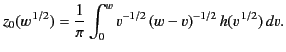
for  . Let us multiply both sides
of the previous equation by
. Let us multiply both sides
of the previous equation by
 and integrate from
  to
to  .
We obtain
.
We obtain
![$\displaystyle \frac{1}{\pi}\int_0^w v^{-1/2} \,(w-v)^{-1/2} \,h(v^{\,1/2})\,dv ...
...left[\int_0^{z_0(v^{\,1/2})} \! \frac{dz}{(w-v)^{1/2}\, (v-u)^{1/2}}\right] dv.$](img2367.png) |
(1133) |
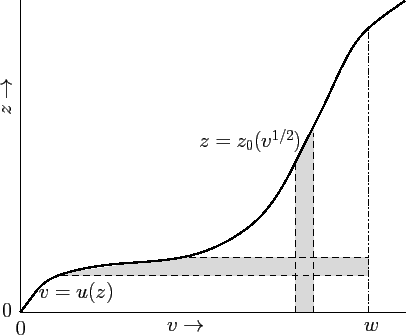
Consider the double integral on the right-hand side of the previous equation. The region
of  -
- space over which this integral is performed is sketched
in Figure 782. It can be seen that, as long as
space over which this integral is performed is sketched
in Figure 782. It can be seen that, as long as
 is
a monotonically increasing function of
, we can swap the order of
integration to give
is
a monotonically increasing function of
, we can swap the order of
integration to give
![$\displaystyle \frac{1}{\pi} \int_0^{z_0(w^{\,1/2})} \left[ \int_{u(z)}^w \frac{dv} {(w-v)^{1/2}\,(v-u)^{1/2}}\right]\,dz.$](img2369.png) |
(1134) |
Here, we have used the fact that the curve
 is identical
with the curve
is identical
with the curve  . Note that if
is not a monotonically
increasing function of
then we can still swap the order of integration, but
the limits of integration are, in general, far more complicated than those
indicated previously. The integral over
in the previous expression can be
evaluated using standard methods (by making the substitution
. Note that if
is not a monotonically
increasing function of
then we can still swap the order of integration, but
the limits of integration are, in general, far more complicated than those
indicated previously. The integral over
in the previous expression can be
evaluated using standard methods (by making the substitution
 ): the result is simply
  . Thus,
expression (1136) reduces to
. Thus,
expression (1136) reduces to
 . It follows from
Equation (1135) that
. It follows from
Equation (1135) that
 |
(1135) |
Making the substitutions
 and
and
 , we obtain
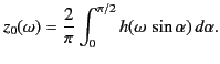 |
(1136) |
By definition,
 at the reflection level
  . Hence,
the previous equation reduces to
. Hence,
the previous equation reduces to
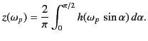 |
(1137) |
Thus, we can obtain
as a function of  (and, hence,
as a
function of
) by simply taking the appropriate integral of
the experimentally determined function
. Because
(and, hence,
as a
function of
) by simply taking the appropriate integral of
the experimentally determined function
. Because
![$ \omega_p(z)
\propto [N(z)]^{1/2}$](img2380.png) , this means that we can determine the electron number density
profile in the ionosphere provided that
we know the variation of the equivalent height
with
pulse frequency. The constraint that
, this means that we can determine the electron number density
profile in the ionosphere provided that
we know the variation of the equivalent height
with
pulse frequency. The constraint that
 must be a
monotonically increasing function of
must be a
monotonically increasing function of  translates to the constraint that
 must be a monotonically increasing function of
.
Note that we can still determine
from
for the case where the
former function is non-monotonic, it is just a far more complicated procedure than
that outlined previously.
Incidentally, the mathematical technique
by which we have inverted Equation (1133), which
specifies
as some integral over
must be a monotonically increasing function of
.
Note that we can still determine
from
for the case where the
former function is non-monotonic, it is just a far more complicated procedure than
that outlined previously.
Incidentally, the mathematical technique
by which we have inverted Equation (1133), which
specifies
as some integral over
 ,
to give
as some integral over
, is known as Abel inversion.
,
to give
as some integral over
, is known as Abel inversion.
Figure:
A sketch of the region of
-
space over which the integral on
the right-hand side of Equation (1133) is evaluated.
 |
Next: Ionospheric Ray Tracing
Up: Wave Propagation in Inhomogeneous
Previous: Ionospheric Pulse Propagation
Richard Fitzpatrick
2014-06-27