Asymptotic Series

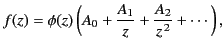
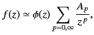
It is often convenient to expand a function of the complex variable $f(z)$ as a series in inverse powers of $z$ . For example,

$$f(z) = \phi(z) \left( A_0 + \frac{A_1}{z} + \frac{A_2}{z^{\,2}}+\cdots\right),$$ (1148)

where $\phi(z)$ is a function whose behavior for large values of $z$ is known. If $f(z)/\phi(z)$ is singular as $\vert z\vert\rightarrow \infty$ then the previous series clearly diverges. Nevertheless, under certain circumstances, the series may still be useful. In fact, this is the case if the difference between $f(z)/\phi(z)$ and the first $n+1$ terms is of order $1/z^{\,n+1}$ , so that for sufficiently large $z$ this difference becomes vanishingly small. More precisely, the series is said to represent $f(z)/\phi(z)$ asymptotically, that is

$$f(z) \simeq \phi(z) \sum_{p=0,\infty} \frac{A_p}{z^{\,p}},$$ (1149)

provided that

$$\lim_{\vert z\vert\rightarrow\infty} \left( z^{\,n} \left[ \frac{f(z)}{\phi(z)} - \sum_{p=0,n}\frac{A_p}{z^{\,p}}\right]\right) \rightarrow 0.$$ (1150)

In other words, for a given value of $n$ , the sum of the first $n+1$ terms of the series may be made as close as desired to the ratio $f(z)/\phi(z)$ by making $z$ sufficiently large. For each value of $z$ and $n$ there is an error in the series representation of $f(z)/\phi(z)$ which is of order $1/z^{\,n+1}$ . Because the series actually diverges, there is an optimum number of terms in the series used to represent $f(z)/\phi(z)$ for a given value of $z$ . Associated with this is an unavoidable error. As $z$ increases, the optimal number of terms increases, and the error decreases.

Consider a simple example. The exponential integral is defined

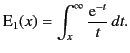$${\rm E}_1(x) = \int_x^\infty \frac{{\rm e}^{-t}}{t}\,dt.$$ (1151)

The asymptotic series for this function can be generated via a series of partial integrations. For example,

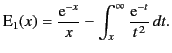$${\rm E}_1(x) = \frac{{\rm e}^{-x}}{x} -\int_x^\infty \frac{{\rm e}^{-t}}{t^{\,2}}\,dt.$$ (1152)

A continuation of this procedure yields

$${\rm E}_1(x) = \frac{{\rm e}^{-x}}{x}\left[ 1-\frac{1}{x} + \frac... ...\,n}}\right] +(-1)^{n+1}(n+1)!\int_x^\infty \frac{{\rm e}^{-t}}{t^{\,n+2}}\,dt.$$ (1153)

The infinite series obtained by taking the limit $n\rightarrow \infty$ diverges, because the Cauchy convergence test yields

$$\lim_{n\rightarrow\infty} \left\vert\frac{u_{n+1}}{u_n}\right\vert =\lim_{n\rightarrow\infty} \left(\frac{n}{x}\right)\rightarrow\infty.$$ (1154)

Note that two successive terms in the series become equal in magnitude for $n=x$ , indicating that the optimum number of terms for a given $x$ is roughly the nearest integer to $x$ . To prove that the series is asymptotic, we need to show that

$$\lim_{x\rightarrow 0}\,x^{\,n+1}\,{\rm e}^{\,x}\, (-1)^{n+1}\,(n+1)!\int_x^\infty \frac{{\rm e}^{-t}}{t^{\,n+2}} \,dt = 0.$$ (1155)

This immediately follows, because

$$\int_x^{\infty} \frac{{\rm e}^{-t}}{t^{\,n+2}} \,dt < \frac{1}{x^{\,n+2}}\int_x^\infty {\rm e}^{-t} \,dt = \frac{{\rm e}^{-x}} {x^{\,n+2}}.$$ (1156)

Thus, the error involved in using the first $n$ terms in the series is less than $(n+1)! \,{\rm e}^{-x}/x^{\,n+2}$ , which is the magnitude of the next term in the series. We can see that, as $n$ increases, this estimate of the error first decreases, and then increases without limit. In order to visualize this phenomenon more exactly, let $f(x) = x\, \exp(x)\,{\rm E}(x)$ , and let

$$f_n(x) = \sum_{p=0,n}\frac{(-1)^p p!}{x^{\,p}}$$ (1157)

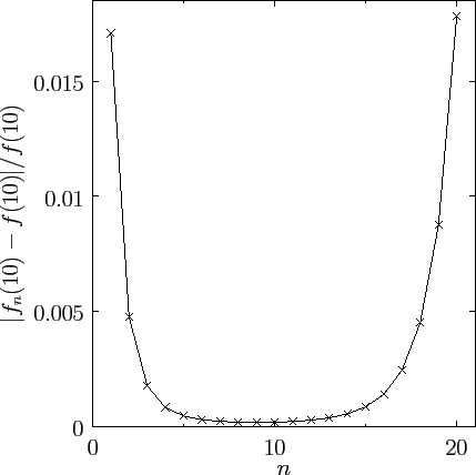
be the asymptotic series representation of this function that contains $n+1$ terms. Figure 21 shows the relative error in the asymptotic series $\vert f_n(x) - f(x)\vert/f(x)$ plotted as a function of the approximate number of terms in the series, $n$ , for $x=10$ . It can be seen that as $n$ increases the error initially falls, reaches a minimum value at about $n=10$ , and then increases rapidly. Clearly, the optimum number of terms in the asymptotic series used to represent $f(10)$ is about 10.

Figure 21: The relative error in a typical asymptotic series plotted as a function of the number of terms in the series.

Asymptotic series are fundamentally different to conventional power law expansions, such as

$$\sin z = z - \frac{z^{\,3}}{3!} + \frac{z^{\,5}}{5!} -\frac{z^{\,7}}{7!} + \cdots .$$ (1158)

This series representation of $\sin z$ converges absolutely for all finite values of $z$ . Thus, at any $z$ , the error associated with the series can be made as small as is desired by including a sufficiently large number of terms. In other words, unlike an asymptotic series, there is no intrinsic, or unavoidable, error associated with a convergent series. It follows that a convergent power law series representation of a function is unique within the domain of convergence of the series. On the other hand, an asymptotic series representation of a function is not unique. It is perfectly possible to have two different asymptotic series representations of the same function, as long as the difference between the two series is less than the intrinsic error associated with each series. Furthermore, it is often the case that different asymptotic series are used to represent the same single-valued analytic function in different regions of the complex plane.

For example, consider the asymptotic expansion of the confluent hypergeometric function $F(a,c,z)$ . This function is the solution of the differential equation

$$z\, F'' +(c-z)\,F' - a \,F = 0$$ (1159)

which is analytic at $z=0$ [in fact, $F(a,c,0)=1$ ]. Here, $'$ denotes $d/dz$ . The asymptotic expansion of $F(a,c,z)$ takes the form:

$$\frac{{\mit\Gamma}(a)\,{\mit\Gamma}(c-a)}{{\mit\Gamma}(c)} \,F(a,... ...a} \,{\rm e}^{-{\rm i}\,\pi\, a}\left[1+{\cal O}\left(\frac{1}{z}\right)\right]$$ (1160)

for $-\pi < {\rm arg}(z) < 0$ , and

$$\frac{{\mit\Gamma}(a)\,{\mit\Gamma}(c-a)}{{\mit\Gamma}(c)} \,F(a,... ...}\, {\rm e}^{\,{\rm i}\,\pi\, a}\left[1+{\cal O}\left(\frac{1}{z}\right)\right]$$ (1161)

for $0 < {\rm arg}(z) < \pi$ , and

$$\frac{{\mit\Gamma}(a)\,{\mit\Gamma}(c-a)}{{\mit\Gamma}(c)} \,F(a,c,z) \simeq {\mit\Gamma}(c-a)\,z^{\,a-c}\, {\rm e}^{-{\rm i}\, 2\pi\,(a-c)} \,{\rm e}^{\,z}\left[1+{\cal O}\left(\frac{1}{z}\right)\right]$$

$$\phantom{=} +{\mit\Gamma}(a)\,z^{-a}\, {\rm e}^{\,{\rm i}\,\pi\, a}\left[1+{\cal O}\left(\frac{1}{z}\right)\right]$$ (1162)

for $\pi < {\rm arg}(z) < 2\pi$ , et cetera. Here,

$${\mit\Gamma}(z)= \int_0^\infty t^{\,z-1}\,{\rm e}^{-t}\,dt$$ (1163)

is a so-called Gamma function. This function has the property that ${\mit\Gamma}(n+1)=n!$ , where $n$ is a non-negative integer. It can be seen that the expansion consists of a linear combination of two asymptotic series (only the first term in each series is shown). For $\vert z\vert\gg 1$ , the first series is exponentially larger than the second whenever ${\rm Re}(z) > 0$ . The first series is said to be dominant in this region, whereas the second series is said to be subdominant. Likewise, the first series is exponentially smaller than the second whenever ${\rm Re}(z) < 0$ . Hence, the first series is subdominant, and the second series dominant, in this region.

Consider a region in which one or other of the series is dominant. Strictly speaking, it is not mathematically consistent to include the subdominant series in the asymptotic expansion, because its contribution is actually less than the intrinsic error associated with the dominant series [this error is ${\cal O}(1/z)$ times the dominant series, because we are only including the first term in this series]. Thus, at a general point in the complex plane, the asymptotic expansion simply consists of the dominant series. However, this is not the case in the immediate vicinity of the lines ${\rm Re}(z)= 0$ , which are called anti-Stokes lines. When an anti-Stokes line is crossed, a dominant series becomes subdominant, and vice versa. Thus, in the immediate vicinity of an anti-Stokes line neither series is dominant, so it is mathematically consistent to include both series in the asymptotic expansion.

The hypergeometric function $F(a,c,z)$ is a perfectly well-behaved, single-valued, analytic function in the complex plane. However, our two asymptotic series are, in general, multi-valued functions in the complex plane [see Equation (1162)]. Can a single-valued function be represented asymptotically by a multi-valued function? The short answer is no. We have to employ different combinations of the two series in different regions of the complex plane in order to ensure that $F(a,c,z)$ remains single-valued. Equations (1162)-(1164) show how this is achieved. Basically, the coefficient in front of the subdominant series changes discontinuously at certain values of ${\rm arg}(z)$ . This is perfectly consistent with $F(a,c,z)$ being an analytic function because the subdominant series is ``invisible'': in other words, the contribution of the subdominant series to the asymptotic solution falls below the intrinsic error associated with the dominant series, so that it does not really matter if the coefficient in front of the former series changes discontinuously. Imagine tracing a large circle, centered on the origin, in the complex plane. Close to an anti-Stokes line, neither series is dominant, so we must include both series in the asymptotic expansion. As we move away from the anti-Stokes line, one series becomes dominant, which means that the other series becomes subdominant, and, therefore, drops out of our asymptotic expansion. Eventually, we approach a second anti-Stokes line, and the subdominant series reappears in our asymptotic expansion. However, the coefficient in front of the subdominant series, when it reappears, is different to that when the series disappeared. This new coefficient is carried across the second anti-Stokes line into the region where the subdominant series becomes dominant. In this new region, the dominant series becomes subdominant, and disappears from our asymptotic expansion. Eventually, a third anti-Stokes line is approached, and the series reappears, but, again, with a different coefficient in front. The jumps in the coefficients of the subdominant series are chosen in such a manner that if we perform a complete circuit in the complex plane then the value of the asymptotic expansion is the same at the beginning and the end points. In other words, the asymptotic expansion is single-valued, despite the fact that it is built up out of two asymptotic series that are not single-valued. The jumps in the coefficient of the subdominant series, which are needed to keep the asymptotic expansion single-valued, are called Stokes phenomena, after the celebrated nineteenth century British mathematician Sir George Gabriel Stokes, who first drew attention to this effect.

Where exactly does the jump in the coefficient of the subdominant series occur? All we can really say is ``somewhere in the region between two anti-Stokes lines where the series in question is subdominant.'' The problem is that we only retained the first term in each asymptotic series. Consequently, the intrinsic error in the dominant series is relatively large, and we lose track of the subdominant series very quickly after moving away from an anti-Stokes line. However, we could include more terms in each asymptotic series. This would enable us to reduce the intrinsic error in the dominant series, and, thereby, expand the region of the complex plane in the vicinity of the anti-Stokes lines where we can see both the dominant and subdominant series. If we were to keep adding terms to our asymptotic series, so as to minimize the error in the dominant solution, we would eventually be forced to conclude that a jump in the coefficient of the subdominant series can only take place on those lines in the complex plane on which ${\rm Im }(z)=0$ : these are called Stokes lines. This result was first proved by Stokes in 1857.On a Stokes line, the magnitude of the dominant series achieves its maximum value with respect to that of the subdominant series. Once we know that a jump in the coefficient of the subdominant series can only take place at a Stokes line, we can retain the subdominant series in our asymptotic expansion in all regions of the complex plane. What we are basically saying is that, although, in practice, we cannot actually see the subdominant series very far away from an anti-Stokes line, because we are only retaining the first term in each asymptotic series, we could, in principle, see the subdominant series at all values of ${\rm arg}(z)$ provided that we retained a sufficient number of terms in our asymptotic series.

Figure 22: The location of the Stokes lines (dashed), the anti-Stokes lines (solid), and the branch cut (wavy) in the complex plane for the asymptotic expansion of the hypergeometric function.

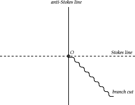Figure 784 shows the location in the complex plane of the Stokes and anti-Stokes lines for the asymptotic expansion of the hypergeometric function. Also shown is a branch cut, which is needed to make $z$ single-valued. The branch cut is chosen such that ${\rm arg}(z)=0$ on the positive real axis. Every time we cross an anti-Stokes line, the dominant series becomes subdominant, and vice versa. Every time we cross a Stokes line, the coefficient in front of the dominant series stays the same, but that in front of the subdominant series jumps discontinuously [see Equations (1162)-(1164)]. Finally, the jumps in the coefficient of the subdominant series are such as to ensure that the asymptotic expansion is single-valued.