


Next: Propagation in a conductor
Up: Electromagnetic radiation
Previous: Dielectric constant of a
Consider a high frequency electromagnetic wave propagating, along the  -axis, through
a plasma with a longitudinal equilibrium magnetic field,
-axis, through
a plasma with a longitudinal equilibrium magnetic field,
 .
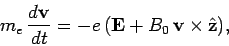
The equation of motion of an individual electron making up the plasma takes the
form
.
The equation of motion of an individual electron making up the plasma takes the
form
 |
(1166) |
where the first term on the right-hand side is due to the wave electric field,
and the second to the equilibrium magnetic field.
(As usual, we can neglect the wave magnetic field, provided that the
electron motion remains non-relativistic.)
Of course,
 , where
  is the electron
displacement from its equilibrium position. Suppose that all perturbed quantities vary with time
like
is the electron
displacement from its equilibrium position. Suppose that all perturbed quantities vary with time
like
 , where
  is the wave frequency.
It follows that
is the wave frequency.
It follows that
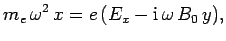 |
|
|
(1167) |
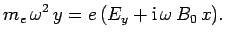 |
|
|
(1168) |
It is helpful to define
Using these new variables, Eqs. (1167) and (1168)
can be rewritten
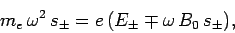 |
(1171) |
which can be solved to give
 |
(1172) |
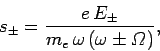
where
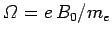 is the so-called cyclotron frequency (i.e.,
the characteristic gyration frequency of free electrons in the
equilibrium magnetic field--see Sect. 3.7).
is the so-called cyclotron frequency (i.e.,
the characteristic gyration frequency of free electrons in the
equilibrium magnetic field--see Sect. 3.7).
In terms of  , the electron displacement can be written
 |
(1173) |
where
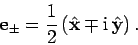 |
(1174) |
Likewise, in terms of  , the wave electric field takes the form
 |
(1175) |
Obviously, the actual displacement and electric field are the real
parts of the above expressions. It follows from Eq. (1175)
that  corresponds to a constant amplitude electric field which rotates anti-clockwise
in the
corresponds to a constant amplitude electric field which rotates anti-clockwise
in the  -
- plane (looking down the -axis) as the wave propagates in the
  -direction, whereas
 corresponds to a constant amplitude electric field which rotates clockwise.
The former type of wave is termed right-hand circularly polarized,
whereas the latter is termed left-hand circularly polarized.
Note also that
corresponds to a constant amplitude electric field which rotates clockwise.
The former type of wave is termed right-hand circularly polarized,
whereas the latter is termed left-hand circularly polarized.
Note also that  and
and  correspond to circular electron motion
in opposite senses.
With these insights, we conclude that Eq. (1172) indicates that
individual electrons in the plasma have a slightly different response to right- and left-hand circularly polarized waves in the presence of a
longitudinal magnetic field.
correspond to circular electron motion
in opposite senses.
With these insights, we conclude that Eq. (1172) indicates that
individual electrons in the plasma have a slightly different response to right- and left-hand circularly polarized waves in the presence of a
longitudinal magnetic field.
Following the analysis of Sect. 9.7, we can deduce from Eq. (1172) that the dielectric constant of the plasma for right- and
left-hand circularly
polarized waves is
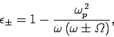 |
(1176) |
respectively. Hence, according to Eq. (1154), the dispersion relation
for right- and left-hand circularly polarized waves becomes
![\begin{displaymath}
k_{\pm}^{ 2} c^2 = \omega^2\left[1- \frac{\omega_p^{ 2}}{\omega (\omega\pm{\mit \Omega})}\right],
\end{displaymath}](img2376.png) |
(1177) |
respectively.
In the limit
 , we obtain
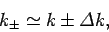 |
(1178) |
where
![$k= \omega [1-(1/2) \omega_p^{ 2}/\omega^2]/c$](img2379.png) and
and
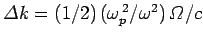 . In other words, in a magnetized plasma,
right- and left-hand circularly polarized waves of the same frequency have
slightly different wave-numbers
. In other words, in a magnetized plasma,
right- and left-hand circularly polarized waves of the same frequency have
slightly different wave-numbers
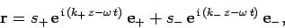
Let us now consider the propagation of a linearly polarized electromagnetic
wave through the plasma. Such a wave can be constructed via a superposition
of right- and left-hand circularly polarized waves of equal
amplitudes. So, the wave electric field can be written
![\begin{displaymath}
{\bf E} = E_0 \left[{\rm e}^{ {\rm i} (k_+ z-\omega t)}\...
...
+ {\rm e}^{ {\rm i} (k_- z-\omega t)} {\bf e}_- \right].
\end{displaymath}](img2381.png) |
(1179) |
It can easily be seen that at  the wave electric field is aligned
along the -axis. If right- and left-hand circularly polarized waves
of the same frequency have the same wave-number (i.e., if
the wave electric field is aligned
along the -axis. If right- and left-hand circularly polarized waves
of the same frequency have the same wave-number (i.e., if
 ) then the wave electric field will continue to be aligned
along the -axis as the wave propagates in the -direction:
i.e., we will have a standard linearly polarized wave. However, we have just
demonstrated
that, in the presence of a longitudinal magnetic field, the wave-numbers
) then the wave electric field will continue to be aligned
along the -axis as the wave propagates in the -direction:
i.e., we will have a standard linearly polarized wave. However, we have just
demonstrated
that, in the presence of a longitudinal magnetic field, the wave-numbers  and
and  are slightly different. What effect does this have on the polarization of the
wave?
are slightly different. What effect does this have on the polarization of the
wave?
Taking the real part of Eq. (1179), and making use of Eq. (1178), and some standard trigonometrical identities,
we obtain
![\begin{displaymath}
{\bf E} =E_0 \left[\cos(k z-\omega t) \cos({\mit\Delta} k...
...,
\cos(k z-\omega t) \sin({\mit\Delta} k z), 0\right].
\end{displaymath}](img2385.png) |
(1180) |
The polarization angle of the wave (which is a convenient measure of
its plane of polarization) is given by
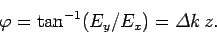 |
(1181) |
Thus, we conclude that in the presence of a longitudinal magnetic field
the polarization angle rotates as as the wave propagates through the plasma. This effect is
known as Faraday rotation. It is clear, from the above expression,
that the rate of advance of the polarization angle with distance
travelled by the wave is given by
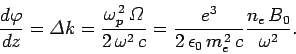 |
(1182) |
Hence, a linearly polarized electromagnetic wave which propagates through a
plasma with a (slowly) varying electron number density,  ,
and longitudinal magnetic field,
,
and longitudinal magnetic field,  , has its plane of
polarization rotated through a total angle
, has its plane of
polarization rotated through a total angle
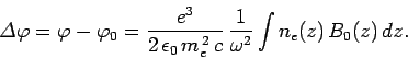 |
(1183) |
Note the very strong inverse variation of
 with .
Pulsars are rapidly rotating neutron stars which emit regular blips of
highly polarized radio waves. Hundreds of such objects have been found
in our galaxy since the first was discovered in 1967. By measuring
the variation of the angle of polarization,  , of radio emission from a pulsar with frequency, , astronomers can effectively determine
the line integral of
, of radio emission from a pulsar with frequency, , astronomers can effectively determine
the line integral of  along the straight-line joining the
pulsar to the Earth using formula (1183). Here,
along the straight-line joining the
pulsar to the Earth using formula (1183). Here,  is the number
density of free electrons in the interstellar medium, whereas
is the number
density of free electrons in the interstellar medium, whereas  is the parallel component of the galactic magnetic field. Obviously, in order
to achieve this, astronomers must make the reasonable assumption that the
radiation was emitted by the pulsar with a common angle of polarization,
is the parallel component of the galactic magnetic field. Obviously, in order
to achieve this, astronomers must make the reasonable assumption that the
radiation was emitted by the pulsar with a common angle of polarization,  ,
over a wide range of different frequencies. By fitting Eq. (1183)
to the data, and then extrapolating to large , it is then possible to
determine , and, hence, the amount,
,
over a wide range of different frequencies. By fitting Eq. (1183)
to the data, and then extrapolating to large , it is then possible to
determine , and, hence, the amount,
 ,
through which the polarization angle of the radiation has rotated, at a given frequency, during its passage to Earth.
,
through which the polarization angle of the radiation has rotated, at a given frequency, during its passage to Earth.
Next: Propagation in a conductor
Up: Electromagnetic radiation
Previous: Dielectric constant of a
Richard Fitzpatrick
2006-02-02