Next: Effect of solar radiation Up: Secular perturbation theory Previous: Effect of terrestrial oblateness
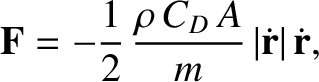
The force per unit mass that the atmosphere exerts on an orbiting satellite can be modeled as (Batchelor 2000)
where is the mass density of the atmosphere (at the satellite's position),
  the drag coefficient,
  the cross-sectional area of the satellite perpendicular to its direction of motion,
  the satellite mass,
and
the satellite mass,
and
 the satellite velocity. It can be seen that the
force is proportional to the square of the satellite speed, and is oppositely directed to its instantaneous direction of motion (i.e., the force constitutes a drag).
The drag coefficient is an order unity dimensionless constant that depends primarily on the satellite's shape. For the case of a spherical
satellite,
the satellite velocity. It can be seen that the
force is proportional to the square of the satellite speed, and is oppositely directed to its instantaneous direction of motion (i.e., the force constitutes a drag).
The drag coefficient is an order unity dimensionless constant that depends primarily on the satellite's shape. For the case of a spherical
satellite,
 (Cook 1965).
The density distribution of the terrestrial atmosphere is conveniently modeled as (de Pater and Lissauer 2010)
![$\displaystyle \rho(r) = \rho_0\exp\left[-\frac{(r-R)}{H}\right],$](img2733.png) |
(10.131) |
 measures radial distance from the Earth's center,
 is the terrestrial radius,
 the
atmospheric density at ground level (i.e.,
the
atmospheric density at ground level (i.e.,  ), and
 the atmospheric scale height. Obviously, the previous formula is only valid when
  .
.
Assuming that the atmospheric drag force, (10.130), is small compared to the force of gravitational attraction between the Earth and the
satellite—and can, thus, be treated as a perturbation—the satellite's orbit can be modeled as Keplerian ellipse whose six elements evolve
slowly in time under the influence of the drag.
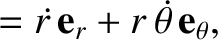
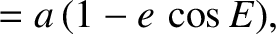
Let ,  ,
,  be cylindrical coordinates in a reference frame that is aligned with the satellite's instantaneous orbital plane, as
described in Section I.1. Here, is the satellite's true anomaly. (See Section 4.11.) Making use of the analysis
of Appendix I, we can write
be cylindrical coordinates in a reference frame that is aligned with the satellite's instantaneous orbital plane, as
described in Section I.1. Here, is the satellite's true anomaly. (See Section 4.11.) Making use of the analysis
of Appendix I, we can write
 |
 |
(10.132) |
 |
 |
(10.133) |
 |
 |
(10.134) |
 |
 |
(10.135) |
 |
 |
(10.136) |
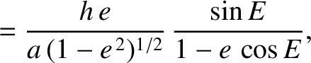
 ,
,  ,
,  , and
, and  are the satellite's orbital major radius, eccentricity, angular momentum per unit mass, and
eccentric anomaly, respectively. (See Section 4.11.) Moreover,
are the satellite's orbital major radius, eccentricity, angular momentum per unit mass, and
eccentric anomaly, respectively. (See Section 4.11.) Moreover,
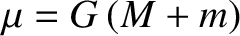 , where
  is the terrestrial mass.
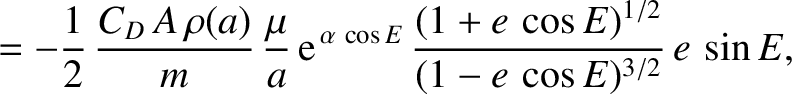
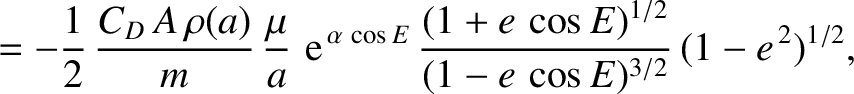
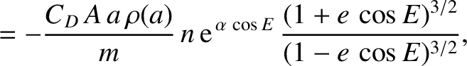
It follows from the previous equations that
where
is the terrestrial mass.
It follows from the previous equations that
where
 .
.
As has already been mentioned, the satellite's instantaneous orbit is a Keplerian ellipse characterized by six orbital elements, which we
choose to be the major radius, , the mean anomaly at epoch,
 , the eccentricity, , the argument of the perigee,
  ,
the inclination (to the Earth's equatorial plane),
,
the inclination (to the Earth's equatorial plane),  , and the longitude of the ascending node (measured with respect to the vernal equinox),
 .
(See Section 4.12.) These elements evolve slowly in time, under the influence of the atmospheric drag force. For the case in hand, this time evolution is most
conveniently specified in terms of the Gauss planetary equations, which take the form (see Appendix I)
.
(See Section 4.12.) These elements evolve slowly in time, under the influence of the atmospheric drag force. For the case in hand, this time evolution is most
conveniently specified in terms of the Gauss planetary equations, which take the form (see Appendix I)
 |
![$\displaystyle = \frac{2\,h}{\mu\,(1-e^{\,2})}\left[e\,\sin\theta\,F_r + (1+e\,\cos\theta)\,F_\theta\right],$](img2754.png) |
(10.140) |
 |
![$\displaystyle = \frac{h}{\mu}\,\frac{(1-e^{\,2})^{1/2}}{e}\left(\left[\cos\thet...
... -\left[1+\frac{1}{(1-e^{\,2})}\,\frac{r}{a}\right]\sin\theta\,F_\theta\right),$](img2756.png) |
(10.141) |
 |
![$\displaystyle = \frac{h}{\mu}\left[\sin\theta\,F_r+(\cos\theta+\cos E)\,F_\theta \right],$](img2758.png) |
(10.142) |
 |
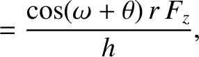
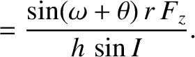
![$\displaystyle = -\frac{h}{\mu}\,\frac{1}{e}\left[\cos\theta\,F_r-\left(\frac{2+...
...theta\,F_\theta \right] -\frac{\cos I\,\sin(\omega+\theta)\,r\,F_z}{h\,\sin I},$](img2760.png) |
(10.143) |
 |
 |
(10.144) |
 |
 |
(10.145) |
 |
 |
(10.146) |
 |
 |
(10.147) |
 is the unperturbed mean orbital angular velocity.
It is immediately apparent that the atmospheric drag force does not give rise to any change in the inclination of the satellite's orbital
plane (because and
are both constant). This is not surprising, because the drag force has no component
normal to this plane (i.e.,
is the unperturbed mean orbital angular velocity.
It is immediately apparent that the atmospheric drag force does not give rise to any change in the inclination of the satellite's orbital
plane (because and
are both constant). This is not surprising, because the drag force has no component
normal to this plane (i.e.,  ).
).
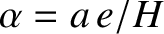
As explained previously, we are working in the limit in which the atmospheric drag force is perturbative. This limit requires the
relative changes in the satellite's orbital elements induced by the drag in an orbital period,  , to all be small. It is apparent from
Equations (10.148)–(10.151) that this is the case provided
, to all be small. It is apparent from
Equations (10.148)–(10.151) that this is the case provided
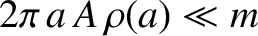 ; in other words, as long as the
mass of air encountered by the satellite in a single orbit, which is
; in other words, as long as the
mass of air encountered by the satellite in a single orbit, which is
 , is much less than the satellite's mass.
Assuming that we are in the perturbative limit (i.e.,
), the evolution of the satellite's orbital elements takes place on a timescale that is
much longer than its orbital period. We can concentrate on this evolution, and filter out any
relatively short-term oscillations in the elements, by averaging expressions (10.148)–(10.151) over an
orbital period. A suitable orbit-average operator is
, is much less than the satellite's mass.
Assuming that we are in the perturbative limit (i.e.,
), the evolution of the satellite's orbital elements takes place on a timescale that is
much longer than its orbital period. We can concentrate on this evolution, and filter out any
relatively short-term oscillations in the elements, by averaging expressions (10.148)–(10.151) over an
orbital period. A suitable orbit-average operator is
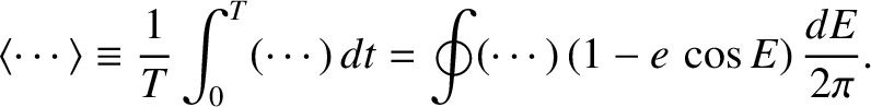 |
(10.154) |
 , and
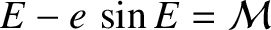
, and
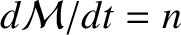 , for a
Keplerian orbit. (See Section 4.11.)
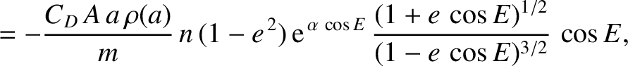
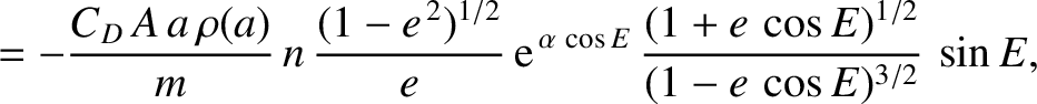
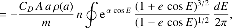
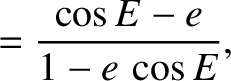
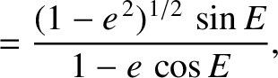
Thus, we deduce that
It follows that the atmospheric drag force causes the major radius and eccentricity of the satellite's orbit to both decay
monotonically in time [because the right-hand sides of Equations (10.155) and (10.156) are both negative]. On the other hand, the force does not produce any precession in the perigee of the orbit (because
, for a
Keplerian orbit. (See Section 4.11.)
Thus, we deduce that
It follows that the atmospheric drag force causes the major radius and eccentricity of the satellite's orbit to both decay
monotonically in time [because the right-hand sides of Equations (10.155) and (10.156) are both negative]. On the other hand, the force does not produce any precession in the perigee of the orbit (because
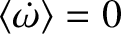 ). Furthermore, the fact that
 implies that the drag force does not modify the Keplerian result that the mean orbital angular velocity is
 .
Now, it is easily demonstrated (see Exercise 4) that the satellite's orbit-averaged kinetic energy is
.
Now, it is easily demonstrated (see Exercise 4) that the satellite's orbit-averaged kinetic energy is
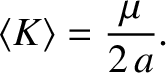 |
(10.159) |
decreases). Evidently, the negative work done on the satellite by the drag force is
more than offset by the positive work done by gravity as its altitude decreases.