Spin-orbit coupling
Let us investigate the spinning motion (i.e., the rotational motion about an axis passing through the center of mass) of an aspherical moon in a Keplerian elliptical orbit about a spherically symmetric planet of mass  . It is
convenient to analyze this motion in a frame of reference whose origin always coincides with the moon's center of
mass,
. It is
convenient to analyze this motion in a frame of reference whose origin always coincides with the moon's center of
mass,  . Let us define a Cartesian coordinate system
  ,
,  ,
,  whose axes are aligned with the moon's principal axes of rotation, and let
 ,
,
 ,
,
 be the corresponding principal moments of inertia. Suppose that
 ,
which implies that the moon's radius attains its greatest and least values at those points where the - and -axes pierce its surface, respectively (assuming that the moon's shape is roughly ellipsoidal).
Let the
planet,
,
which implies that the moon's radius attains its greatest and least values at those points where the - and -axes pierce its surface, respectively (assuming that the moon's shape is roughly ellipsoidal).
Let the
planet,  , be located at position vector
 , ,
, ,  . We can treat the planet as a
point mass, because it is
spherically symmetric. Incidentally, we are assuming that the moon's deviations from spherical symmetry are
of a permanent nature, being maintained by internal tensile strength, rather than being induced by tidal or
rotational effects.
. We can treat the planet as a
point mass, because it is
spherically symmetric. Incidentally, we are assuming that the moon's deviations from spherical symmetry are
of a permanent nature, being maintained by internal tensile strength, rather than being induced by tidal or
rotational effects.
According to MacCullagh's formula, the gravitational potential produced at by the
gravitational field of the moon is (see Section 8.9)
 |
(8.146) |
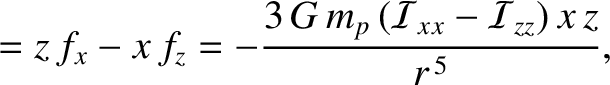
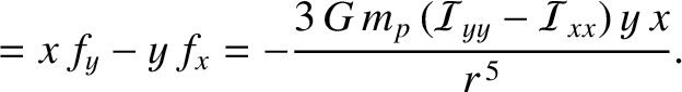
Thus, the gravitational force,  , exerted on the planet by the moon has the components
Furthermore, the components of the torque,
, exerted on the planet by the moon has the components
Furthermore, the components of the torque,
 , acting on the planet about point are
Of course, an equal and opposite torque,
, acting on the planet about point are
Of course, an equal and opposite torque,
 , acts on the moon.
Euler's equation for the moon's spinning motion take the form (see Section 8.6)
where

 ,
,  ,
,  is the associated angular velocity vector.
Suppose that the moon is actually spinning about the -axis (i.e., the principal axis of rotation with the
largest associated moment of inertia), and that this axis is directed
normal to the moon's orbital plane (which is assumed to be fixed). It follows that
where
is the associated angular velocity vector.
Suppose that the moon is actually spinning about the -axis (i.e., the principal axis of rotation with the
largest associated moment of inertia), and that this axis is directed
normal to the moon's orbital plane (which is assumed to be fixed). It follows that
where  is the relative position angle of the planet in the - plane. See Figure 8.7.
We can write
is the relative position angle of the planet in the - plane. See Figure 8.7.
We can write
 , where
  is the angle subtended between the -axis (say)
and some fixed (with respect to distant stars) direction in the --plane. Let this direction be parallel to the
major axis
is the angle subtended between the -axis (say)
and some fixed (with respect to distant stars) direction in the --plane. Let this direction be parallel to the
major axis
 of the moon's orbit, where
  is the pericenter (i.e., the point of closest approach of the moon
to the planet). In this case, it is clear from Figure 8.7 that
is the pericenter (i.e., the point of closest approach of the moon
to the planet). In this case, it is clear from Figure 8.7 that
 |
(8.158) |
where  is the moon's orbital true anomaly. (See Chapter 4.) Hence, Equations (8.152), (8.155),
(8.156), and (8.157) yield
is the moon's orbital true anomaly. (See Chapter 4.) Hence, Equations (8.152), (8.155),
(8.156), and (8.157) yield
![$\displaystyle \skew{5}\ddot{\phi}+\frac{3}{2}\,n^{\,2}\left(\frac{{\cal I}_{yy}...
...{xx}}{{\cal I}_{zz}}\right)\left(\frac{a}{r}\right)^3
\sin[2\,(\phi-\theta)]=0,$](img1850.png) |
(8.159) |
where use has been made of the standard Keplerian result
 (assuming that the mass of the moon
is much less than that of the planet). (See Chapter 4.) Here,
(assuming that the mass of the moon
is much less than that of the planet). (See Chapter 4.) Here,  and
and  are the moon's orbital major radius and mean angular
velocity, respectively.
are the moon's orbital major radius and mean angular
velocity, respectively.
Figure 8.7:
Geometry of spin-orbit coupling.
|
|
Assuming that the eccentricity,  , of the moon's orbit is low—so that
 —it follows from
Equations (4.86) and (4.87), as well as the trigonometric inequalities listed in Section A.3,
that
—it follows from
Equations (4.86) and (4.87), as well as the trigonometric inequalities listed in Section A.3,
that
where  is the moon's mean anomaly. Note that
 . Hence, Equation (8.159) gives
where any
. Hence, Equation (8.159) gives
where any
 terms have been neglected. Here, use has again been made of the trigonometric identities in Section A.3.
Suppose that the moon passes through its pericenter at time  , so that
 |
(8.165) |
In this case, the previous equation becomes
![$\displaystyle \frac{d^{\,2}\phi}{dt^{\,2}} \simeq-\frac{n_0^{\,2}}{2}\left[-\fr...
...phi-n\,t)+\sin(2\,\phi-2\,n\,t)
+ \frac{7\,e}{2}\,\sin(2\,\phi-3\,n\,t)\right],$](img1867.png) |
(8.166) |
where the so-called asphericity parameter,
![$\displaystyle \alpha= \left[3\,\left(\frac{{\cal I}_{yy}-{\cal I}_{xx}}{{\cal I}_{zz}}\right)\right]^{1/2},$](img1868.png) |
(8.167) |
is a measure of the moon's departure from spherical symmetry, and
 |
(8.168) |
Figure: 8.8
Surface of section plot for solutions of Equation (8.166) with
 and
and  . The major spin-orbit resonances are
labelled.
. The major spin-orbit resonances are
labelled.
|
|
Equation (8.166) is highly nonlinear in nature. Consequently, it does not posses a general analytic solution.
Fortunately, (8.166) is relatively straightforward to solve numerically. In fact, the solution can be represented
as a trajectory in ,
 ,
,  space. Because Equation (8.166)
is deterministic, a trajectory that corresponds to a unique set of initial conditions cannot intersect
a second trajectory that corresponds to a different set of initial conditions. Unfortunately, it is difficult to visualize
a trajectory in three dimensions. However, we can alleviate this problem by only plotting those points where the trajectory
pierces a set of equally spaced planes normal to the axis.
These planes are located at
space. Because Equation (8.166)
is deterministic, a trajectory that corresponds to a unique set of initial conditions cannot intersect
a second trajectory that corresponds to a different set of initial conditions. Unfortunately, it is difficult to visualize
a trajectory in three dimensions. However, we can alleviate this problem by only plotting those points where the trajectory
pierces a set of equally spaced planes normal to the axis.
These planes are located at
 , where
  is an integer. This procedure is equivalent to projecting the trajectory onto the ,
plane each time the moon passes through its
pericenter. The resulting plot is known as a surface of section. Figure 8.8 shows the surface of section
for a set of trajectories corresponding to a great many different initial conditions. All of the
trajectories are calculated from Equation (8.166) using
and . The relatively small value adopted for the eccentricity, , is consistent
with our earlier assumption that the moon's orbit is nearly circular. On the other hand, the relatively small value adopted
for the asphericity parameter,
is an integer. This procedure is equivalent to projecting the trajectory onto the ,
plane each time the moon passes through its
pericenter. The resulting plot is known as a surface of section. Figure 8.8 shows the surface of section
for a set of trajectories corresponding to a great many different initial conditions. All of the
trajectories are calculated from Equation (8.166) using
and . The relatively small value adopted for the eccentricity, , is consistent
with our earlier assumption that the moon's orbit is nearly circular. On the other hand, the relatively small value adopted
for the asphericity parameter,  , implies that the moon is almost spherical.
It can be seen, from Figure 8.8, that a trajectory corresponding to a given set of initial conditions generates
a series of closely spaced points that trace out a closed curve running roughly parallel to the -axis. Actually, there are two distinct types of curve. The majority of curves extend over
all values of , and represent trajectories for which there is no particular correlation between the moon's
spin and orbital motions. However, a relatively small number of curves only extend over a limited range of values.
These curves represent trajectories for which a resonant interaction between the moon's spin and
orbital motions produces a strong correlation between these two types of motion. The exact resonances correspond to the
centers of the eye-shaped structures which can be seen in Figure 8.8.
The three principal spin-orbit resonances evident in the figure are the 1:2, 1:1, and 3:2 resonances. Here, a
, implies that the moon is almost spherical.
It can be seen, from Figure 8.8, that a trajectory corresponding to a given set of initial conditions generates
a series of closely spaced points that trace out a closed curve running roughly parallel to the -axis. Actually, there are two distinct types of curve. The majority of curves extend over
all values of , and represent trajectories for which there is no particular correlation between the moon's
spin and orbital motions. However, a relatively small number of curves only extend over a limited range of values.
These curves represent trajectories for which a resonant interaction between the moon's spin and
orbital motions produces a strong correlation between these two types of motion. The exact resonances correspond to the
centers of the eye-shaped structures which can be seen in Figure 8.8.
The three principal spin-orbit resonances evident in the figure are the 1:2, 1:1, and 3:2 resonances. Here, a  :
: resonance,
where and are positive integers, is such that times the moon's spin
period is equal to times its orbital period. At such a resonance, the moon's principal axes of rotation
point in the same direction every pericenter passages.
resonance,
where and are positive integers, is such that times the moon's spin
period is equal to times its orbital period. At such a resonance, the moon's principal axes of rotation
point in the same direction every pericenter passages.
Consider the : spin-orbit resonance. It is helpful to define
 |
(8.169) |
where  . Here,
  is minus the angle subtended between the moon's -axis and the
major axis of its orbit every passages through the pericenter. Note that
is minus the angle subtended between the moon's -axis and the
major axis of its orbit every passages through the pericenter. Note that
 at
such passages.
In the vicinity of the resonance, we expect to be a relatively slowly
varying function of time. When expressed in terms of , Equation (8.166) yields
Let us now average the right-hand side of the preceding equation over orbital periods, treating the relatively slowly varying quantity
as a constant.
For the 1:1 resonance, for which
at
such passages.
In the vicinity of the resonance, we expect to be a relatively slowly
varying function of time. When expressed in terms of , Equation (8.166) yields
Let us now average the right-hand side of the preceding equation over orbital periods, treating the relatively slowly varying quantity
as a constant.
For the 1:1 resonance, for which  , we are left with
 |
(8.171) |
This follows because
![$\langle \cos[2\,(p-1)\,n\,t]\rangle=\langle 1\rangle =1$](img1884.png) , when , whereas all of the other averages
over rapidly varying terms are zero;
for example,
, when , whereas all of the other averages
over rapidly varying terms are zero;
for example,
![$\langle\cos[(2\,p-1)\,n\,t]\rangle=\langle\cos( n\,t)\rangle =0$](img1885.png) .
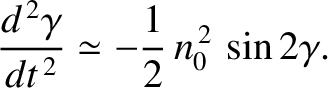
For the 1:2 resonance, for which
.
For the 1:2 resonance, for which  , we are left with
 |
(8.172) |
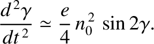
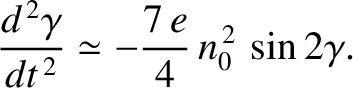
Finally, for the  :
: resonance, for which
  , we are left with
 |
(8.173) |
Figure: 8.9
Contours of  , for
, for
 , plotted in ,
space for the
, plotted in ,
space for the  :, :,
and : spin-orbit resonances. The contours are calculated with
and .
:, :,
and : spin-orbit resonances. The contours are calculated with
and .
|
|
Consider the 1:1 resonance. Multiplying Equation (8.171) by
 , and integrating, we obtain
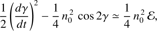 |
(8.174) |
where the constant is related to the moon's spin energy per unit mass. Now,
 .
Furthermore,
.
Furthermore,
 at the times of pericenter passage. Hence, at such times,
 |
(8.175) |
Similar arguments reveal that
 |
(8.176) |
for the : resonance,
and
 |
(8.177) |
for the : resonance.
Figure 8.9 shows contours of plotted in ,
space
for the :, :, and : spin-orbit resonances. These contours are calculated from
Equations (8.175)–(8.177) using
and . It can be seen that the contours shown in Figure 8.9 are very similar to the surface of section curves displayed in Figure 8.8; at least, in the vicinity of the resonances. This suggests that the analytic expressions (8.175)–(8.177) can be used to efficiently map closed surface of section curves in the vicinity of the :, :, and : spin-orbit resonances. Moreover, it is clear, from these expressions, that solutions to Equation (8.166) are
effectively trapped on such curves. This implies that a solution initially close to (say) a : resonance will remain close to this
resonance indefinitely.
For a given spin-orbit resonance, there exists a
separatrix, corresponding to the
 contour, dividing contours that span the whole range
of values from those that only span a restricted range of values. See Figure 8.9. The former contours are
characterized by
contour, dividing contours that span the whole range
of values from those that only span a restricted range of values. See Figure 8.9. The former contours are
characterized by
 ,
whereas the latter are characterized by
,
whereas the latter are characterized by
 . As the energy integral, , is reduced below the
critical value
, the range of allowed values of becomes narrower and narrower. Eventually, when
attains its minimum possible value (i.e.,
. As the energy integral, , is reduced below the
critical value
, the range of allowed values of becomes narrower and narrower. Eventually, when
attains its minimum possible value (i.e.,
 ), is constrained to take a fixed value. This situation corresponds to an exact spin-orbit resonance. For the case of the :
resonance, the minimum energy state corresponds to
), is constrained to take a fixed value. This situation corresponds to an exact spin-orbit resonance. For the case of the :
resonance, the minimum energy state corresponds to  ,
,  and
and
 , which implies that, at the
exact resonance, the moon's -axis points directly toward (or away from) the planet at the
time of pericenter passage. Because we previously assumed that
, which implies that, at the
exact resonance, the moon's -axis points directly toward (or away from) the planet at the
time of pericenter passage. Because we previously assumed that
 , which means that the moon is more elongated
in the -direction than in the -direction, it follows that the long axis (in the - plane) is directed toward the planet each time the moon passes through its pericenter. In this respect, the : resonance is similar to the : resonance.
However, for a moon with a
low-eccentricity orbit locked in a : spin-orbit resonance, the -axis always points
in the general vicinity of the planet, even when the moon is far from its pericenter.
The same is not true for a moon trapped in a : resonance. For the case of the : resonance, the minimum energy state corresponds to
, which means that the moon is more elongated
in the -direction than in the -direction, it follows that the long axis (in the - plane) is directed toward the planet each time the moon passes through its pericenter. In this respect, the : resonance is similar to the : resonance.
However, for a moon with a
low-eccentricity orbit locked in a : spin-orbit resonance, the -axis always points
in the general vicinity of the planet, even when the moon is far from its pericenter.
The same is not true for a moon trapped in a : resonance. For the case of the : resonance, the minimum energy state corresponds to
 and
and
 , which implies that, at the exact resonance, the moon's -axis points directly toward (or away from)
the planet at the time of pericenter passage. In other words, the short axis (in the - plane) is directed toward the planet each time the moon passes through its pericenter.
, which implies that, at the exact resonance, the moon's -axis points directly toward (or away from)
the planet at the time of pericenter passage. In other words, the short axis (in the - plane) is directed toward the planet each time the moon passes through its pericenter.
It can be seen from Equations (8.175)–(8.177)
that the resonance widths (i.e., maximum extent, in the
direction, of the eye-like structure enclosed by the separatrix) of the :, :, and : spin-orbit resonances are  ,
,
 , and
, and
 , respectively.
As long as these widths are significantly less than the inter-resonance spacing (which is
, respectively.
As long as these widths are significantly less than the inter-resonance spacing (which is  ), the three resonances
remain relatively widely separated and are thus distinct from one another. A rough criterion for the
overlap of the : and : resonances is
), the three resonances
remain relatively widely separated and are thus distinct from one another. A rough criterion for the
overlap of the : and : resonances is
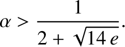 |
(8.178) |
The best example of a celestial body trapped in a : spin-orbit resonance is the planet Mercury, whose
spin period is  days, and whose orbital period is
 days (Yoder 1995). Note that Mercury's axial tilt (with
respect to the normal to its orbital plane) is only
days (Yoder 1995). Note that Mercury's axial tilt (with
respect to the normal to its orbital plane) is only  (Margot et al. 2007). In other words, Mercury is effectively rotating about an
axis that is directed normal to its orbital plane, in accordance with our earlier assumption. It is thought that
Mercury was originally spinning faster than at present, but that its spin rate was gradually
reduced by the tidal de-spinning effect of the Sun (see Section 6.7), until it fell into a : spin-orbit
resonance. As we have seen, once established, such a resonance is maintained by the locking torque exerted by the
Sun on Mercury because of the latter body's small permanent asphericity. However, this is only possible because, close to the resonance, the locking torque exceeds the de-spinning torque.
(Margot et al. 2007). In other words, Mercury is effectively rotating about an
axis that is directed normal to its orbital plane, in accordance with our earlier assumption. It is thought that
Mercury was originally spinning faster than at present, but that its spin rate was gradually
reduced by the tidal de-spinning effect of the Sun (see Section 6.7), until it fell into a : spin-orbit
resonance. As we have seen, once established, such a resonance is maintained by the locking torque exerted by the
Sun on Mercury because of the latter body's small permanent asphericity. However, this is only possible because, close to the resonance, the locking torque exceeds the de-spinning torque.
The best example of a celestial body trapped in a : spin-orbit resonance is the Moon, whose
spin and orbital periods are both  days. The Moon's axial tilt (with respect to the normal
to its orbital plane) is
days. The Moon's axial tilt (with respect to the normal
to its orbital plane) is
 . In other words, the Moon is rotating about an
axis that is (almost) normal to its orbital plane, in accordance with our previous assumption.
Like Mercury, it is thought that the Moon
was originally spinning faster than at present, but that its spin rate was gradually reduced
by tidal de-spinning until it fell into a : spin-orbit resonance. This resonance is
maintained by the locking torque exerted by the Earth on the Moon because of the latter
body's small permanent asphericity, rather than by tidal effects, as
(when the eccentricity of the lunar orbit is taken into account) tidal effects alone would actually cause the
moon's spin rate to exceed its mean orbital rotation rate by about percent (Murray and Dermott 1999).
. In other words, the Moon is rotating about an
axis that is (almost) normal to its orbital plane, in accordance with our previous assumption.
Like Mercury, it is thought that the Moon
was originally spinning faster than at present, but that its spin rate was gradually reduced
by tidal de-spinning until it fell into a : spin-orbit resonance. This resonance is
maintained by the locking torque exerted by the Earth on the Moon because of the latter
body's small permanent asphericity, rather than by tidal effects, as
(when the eccentricity of the lunar orbit is taken into account) tidal effects alone would actually cause the
moon's spin rate to exceed its mean orbital rotation rate by about percent (Murray and Dermott 1999).
Consider a moon whose spin state is close to an exact : spin-orbit resonance. According to the full (i.e., nonaveraged) equation of
motion, Equation (8.170),
 |
(8.179) |
where we have assumed that
 (because the moon is close to the exact resonance), and have also neglected terms of order
  with respect to unity. The preceding equation has
the standard solution
with respect to unity. The preceding equation has
the standard solution
 |
(8.180) |
where  and
and  are arbitrary. This expression is more conveniently written
 |
(8.181) |
From Equations (8.158), (8.161), and (8.169), we have
 |
(8.182) |
which implies that
 |
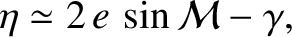
(8.183) |
Here, is the angle subtended between the moon's -axis and the line joining the center of the
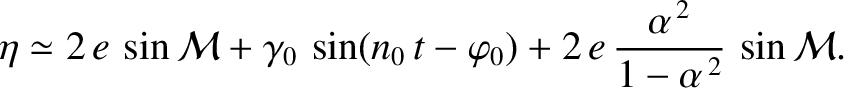
moon to the planet. See Figure 8.7. According to the preceding equation, this angle librates (i.e., oscillates). The first term on the right-hand side of the preceding expression describes so-called optical libration (in longitude). This is
merely a perspective effect due to the eccentricity of the moon's orbit; it does not imply any irregularity in the moon's axial spin rate. The final two terms describe so-called physical libration (in longitude) and are associated with real irregularities in the
moon's spin rate. To be more exact, the first of these terms describes free libration (in longitude), whereas the second
describes forced libration (in longitude). Optical libration causes an oscillation in whose period matches the moon's orbital period, whose amplitude (in radians) is  ,
and whose phase is such that
,
and whose phase is such that  as the moon passes through its pericenter. Forced libration
causes a similar oscillation of much smaller amplitude (assuming that
as the moon passes through its pericenter. Forced libration
causes a similar oscillation of much smaller amplitude (assuming that
 ). Free libration,
on the other hand, causes an oscillation in whose period is
). Free libration,
on the other hand, causes an oscillation in whose period is
 times the
moon's orbital period, and whose amplitude and phase are arbitrary.
times the
moon's orbital period, and whose amplitude and phase are arbitrary.
Consider the Moon, whose spin state is close to a : spin-orbit resonance. According to data from the Lunar Prospector probe (Konopliv et al. 1998; Dickey et al. 1994),
 |
(8.184) |
which implies that
 |
(8.185) |
Hence, given that the Moon's orbital period is  days (i.e., a sidereal month), the predicted
free libration period is
days (i.e., a sidereal month), the predicted
free libration period is  years. Due to the comparatively rapid precession of the Moon's perigee (which completes a
full circuit about the Earth every 8.85 years; see Chapter 11), the expected period of both optical
and forced libration (in longitude) is
years. Due to the comparatively rapid precession of the Moon's perigee (which completes a
full circuit about the Earth every 8.85 years; see Chapter 11), the expected period of both optical
and forced libration (in longitude) is  days (i.e.,
an anomalistic month). Moreover, the predicted amplitudes of these librations are
days (i.e.,
an anomalistic month). Moreover, the predicted amplitudes of these librations are  [when evaluated up to
], and
[when evaluated up to
], and  , respectively.
Optical libration (in longitude) has been observed for hundreds of years, and does indeed have the characteristics described earlier.
Furthermore, despite having an amplitude which is a thousand times less than that of optical
libration, the forced libration (in longitude) of the Moon (due to the eccentricity of the lunar orbit) is measurable by means of laser ranging.
The observed period and amplitude are
days and
, respectively.
Optical libration (in longitude) has been observed for hundreds of years, and does indeed have the characteristics described earlier.
Furthermore, despite having an amplitude which is a thousand times less than that of optical
libration, the forced libration (in longitude) of the Moon (due to the eccentricity of the lunar orbit) is measurable by means of laser ranging.
The observed period and amplitude are
days and  ,
respectively (Williams and Dickey 2003), and are in good agreement with the preceding predictions. Finally, a
free libration (in longitude) mode of the Moon with a period of
,
respectively (Williams and Dickey 2003), and are in good agreement with the preceding predictions. Finally, a
free libration (in longitude) mode of the Moon with a period of  years and an amplitude of
  has been
observed via laser ranging (Jin and Li 1996). The period of this libration is, thus, in good agreement with our
analysis. Note that, because the Moon's orbit has significant non-Keplerian elements, due to the perturbing action of
the Sun, the Moon's forced libration (in longitude) also has important non-Keplerian elements. (See Section 11.18, Exercise 9.)
Furthermore, the Moon also possesses free and forced modes of libration in latitude. (See Section 8.12.)
has been
observed via laser ranging (Jin and Li 1996). The period of this libration is, thus, in good agreement with our
analysis. Note that, because the Moon's orbit has significant non-Keplerian elements, due to the perturbing action of
the Sun, the Moon's forced libration (in longitude) also has important non-Keplerian elements. (See Section 11.18, Exercise 9.)
Furthermore, the Moon also possesses free and forced modes of libration in latitude. (See Section 8.12.)
Figure: 8.10
Surface of section plot for various solutions of Equation (8.166) with the Phobos-like parameters
 and
and  .
.
|
|
The forced libration of the Moon is a tiny effect because of the Moon's relatively small departures from sphericity.
There exist however other moons in the solar system that are locked in a : spin-orbit resonance (like the Moon) and whose departures from sphericity are substantial.
For such moons, forced libration can attain quite large amplitudes.
A prime example is the martian moon Phobos. The shape
of this moon, which is highly irregular (see Figure 3.2), has been measured to high precision by the Mars Express probe,
allowing the computation of the
relative magnitudes of its principal moments of inertia (on the assumption that the moon is
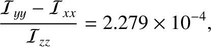
homogeneous). According to this calculation (Wilner at al. 2010),
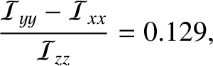 |
(8.186) |
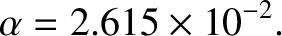
which implies that
 |
(8.187) |
Because the observed eccentricity of Phobos's orbit is (Yoder 1995), the predicted amplitude of its forced physical
libration is  . The measured amplitude is
  (Wilner et al. 2010). Note that the and
values for Phobos
satisfy the resonance overlap criterion in Equation (8.178). Figure 8.10 shows a surface of section plot for Phobos.
It can be seen that resonance overlap leads to the destruction of many of the closed curves that are a feature of
Figure 8.8. Nevertheless, some closed curves remain intact, especially in the vicinity of the :
spin-orbit resonance; that is, around , , and
. Consequently, it is possible for Phobos to
remain close to a : spin-orbit resonant state for an indefinite period of time.
(Wilner et al. 2010). Note that the and
values for Phobos
satisfy the resonance overlap criterion in Equation (8.178). Figure 8.10 shows a surface of section plot for Phobos.
It can be seen that resonance overlap leads to the destruction of many of the closed curves that are a feature of
Figure 8.8. Nevertheless, some closed curves remain intact, especially in the vicinity of the :
spin-orbit resonance; that is, around , , and
. Consequently, it is possible for Phobos to
remain close to a : spin-orbit resonant state for an indefinite period of time.
Figure: 8.11
Surface of section plot for various solutions of Equation (8.166) with the Hyperion-like parameters
 and
and  .
.
|
|
The most extreme example of spin-orbit coupling in the solar system occurs in Hyperion, which is a small
moon of Saturn. Hyperion has a highly irregular shape, with an asphericity parameter of
 |
(8.188) |
(calculated on the assumption that Hyperion is homogeneous),
and is in a fairly eccentric orbit of eccentricity
 |
(8.189) |
(Thomas et al. 1995).
Hence, Hyperion easily satisfies the resonance overlap criterion in Equation (8.178). Figure 8.11 shows
a surface of section plot for Hyperion. It can be seen that resonance overlap leads to the complete destruction of all
of the closed curves associated with the : spin-orbit resonance. This would seem to imply that
Hyperion cannot remain trapped in a : resonance for any appreciable length of time.
Figure 8.12 shows the time evolution of a solution of Equation (8.166), with
Hyperion-like values of and , that starts off in an exact : spin-orbit resonance. If the solution were to stay close to the resonant state then the angle —and, hence,
 —would remain close to zero.
It can be seen, from the figure, that this is not the case. In fact,
quickly becomes of order
unity, indicating a strong deviation from the resonant state. Moreover,
—and, hence,
itself—subsequently varies in a markedly irregular manner. The time variation of is in fact
chaotic; that is, it is quasi-random, never repeats itself, and exhibits extreme sensitivity to initial
conditions (Strogatz 2001). This suggests that Hyperion is spinning in a chaotic manner. Data from the Voyager 2 probe seems to confirm
that this is indeed the case (Black et al. 1995). (Note, however, that Hyperion's
spinning motion involves large chaotic variations in its axial tilt that are not taken into account in our analysis.)
—would remain close to zero.
It can be seen, from the figure, that this is not the case. In fact,
quickly becomes of order
unity, indicating a strong deviation from the resonant state. Moreover,
—and, hence,
itself—subsequently varies in a markedly irregular manner. The time variation of is in fact
chaotic; that is, it is quasi-random, never repeats itself, and exhibits extreme sensitivity to initial
conditions (Strogatz 2001). This suggests that Hyperion is spinning in a chaotic manner. Data from the Voyager 2 probe seems to confirm
that this is indeed the case (Black et al. 1995). (Note, however, that Hyperion's
spinning motion involves large chaotic variations in its axial tilt that are not taken into account in our analysis.)
Figure: 8.12
Solution of Equation (8.166) with the Hyperion-like parameters
and . The
initial conditions are and
. Here,
 .
.
|
|


![$\displaystyle \phantom{=}\left.+ \frac{7\,e}{2}\,\sin(2\,\phi-3\,{\cal M})\right],$](img1864.png)
![\includegraphics[height=4in]{Chapter07/fig7_08.eps}](img1870.png)
![\includegraphics[height=4in]{Chapter07/fig7_09.eps}](img1890.png)
![\includegraphics[height=4in]{Chapter07/fig7_10.eps}](img1939.png)
![\includegraphics[height=4in]{Chapter07/fig7_11.eps}](img1944.png)
![\includegraphics[height=4in]{Chapter07/fig7_12.eps}](img1949.png)


![\includegraphics[height=2.5in]{Chapter07/fig7_07.eps}](img1852.png)

![$\displaystyle \simeq-\frac{n_0^{\,2}}{2}\left[\left(-\frac{e}{2}\,\cos[(2\,p-1)...
...[2\,(p-1)\,n\,t]+\frac{7\,e}{2}\,\cos[(2\,p-3)\,n\,t]\right)\sin 2\gamma\right.$](img1880.png)
![$\displaystyle \phantom{=}\left.+\left(-\frac{e}{2}\,\sin[(2\,p-1)\,n\,t]
+\sin[2\,(p-1)\,n\,t]+\frac{7\,e}{2}\,\sin[(2\,p-3)\,n\,t]\right)\cos 2\gamma\right].$](img1881.png)