MacCullagh's formula
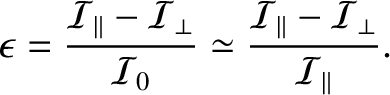
According to Equations (3.59) and (3.64), if the Earth
is modeled as spheroid of uniform density  then its ellipticity
is given by
then its ellipticity
is given by
 |
(8.65) |
where the integral is over the whole volume of the Earth, and
 would be the Earth's moment of inertia were it
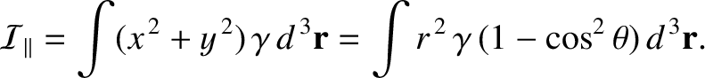
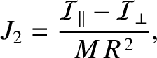
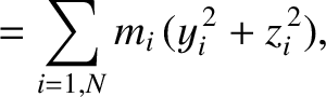
exactly spherical. The Earth's moment of inertia about its
axis of rotation is given by
would be the Earth's moment of inertia were it
exactly spherical. The Earth's moment of inertia about its
axis of rotation is given by
 |
(8.66) |
Here, use has been made of Equations (3.24)–(3.26). Likewise,
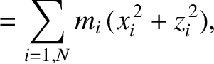
the Earth's moment of inertia about an axis perpendicular to its
axis of rotation (and passing through the Earth's center) is
because the average of
 is
is  for an axisymmetric mass distribution. It follows from the preceding three equations that
 |
(8.68) |
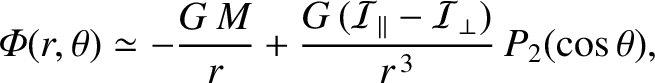
When Equation (8.68) is combined with Equation (3.65), we get
 |
(8.69) |
which is the general expression for the gravitational potential generated outside
an axially symmetric mass distribution. The first term on the right-hand
side is the monopole gravitational potential that would be generated
if all of the mass in the distribution were concentrated at its center of mass,
whereas the second term is the quadrupole potential generated by any deviation from spherical symmetry in the distribution.
Equation (8.69) actually holds for any axially symmetric mass distribution, not just a spheroidal mass distribution of
uniform density (this is discussed in the following).
More generally, consider an asymmetric mass distribution consisting of  mass elements. Suppose that the
 th element has mass
  and
position vector
and
position vector  , where runs from
  to . Let us define a Cartesian coordinate system
  ,
,  ,
,  such that the
origin coincides with the center of mass of the distribution. It follows that
such that the
origin coincides with the center of mass of the distribution. It follows that
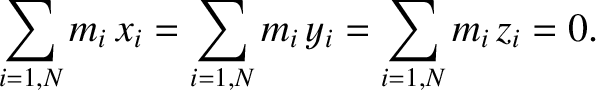 |
(8.70) |
Suppose that the -, -, and -axes coincide with the mass distribution's principal axes of rotation (for rotation
about an axis that passes through the origin). It follows from
Section 8.5 that
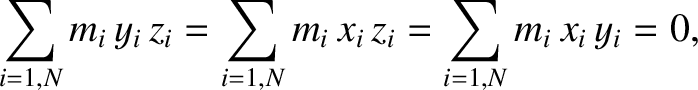 |
(8.71) |
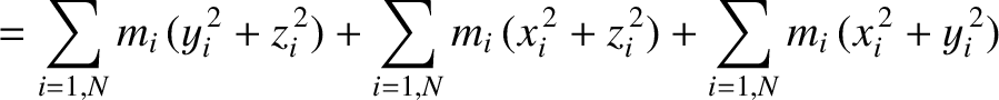
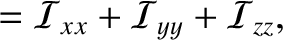
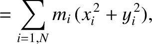
and that the distribution's principal moments of inertia about the -, -, and -axes take the form
respectively.
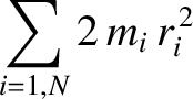
Figure 8.3:
A general mass distribution.
|
|
Consider the gravitational potential,
 , generated by the mass distribution at some external point
  whose position
vector is
whose position
vector is
 , ,
, ,  . According to Section 3.2,
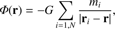 |
(8.75) |
which can also be written
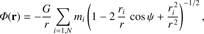 |
(8.76) |
where  is the angle subtended between the vectors
  and . See Figure 8.3. Suppose that
the distance
and . See Figure 8.3. Suppose that
the distance
 is much larger than the characteristic radius of the mass distribution, which implies that
 for all . Expanding up to second order in
  , we obtain
![$\displaystyle {\mit\Phi}({\bf r})\simeq -\frac{G}{r}\sum_{i=1,N}m_i\left[1+\fra...
...si+ \frac{1}{2}\,\frac{r_i^{\,2}}{r^{\,2}}
\left(3\,\cos^2\psi-1\right)\right].$](img1683.png) |
(8.77) |
However,
 |
(8.78) |
where use has been made of Equations (8.70).
Hence, we are left with
 |
(8.79) |
Here,
 is the total mass of the distribution.
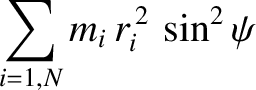
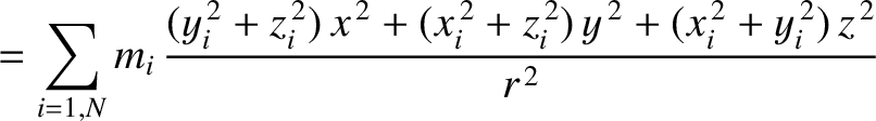
Now,
where use has been made of Equations (8.72)–(8.74). Furthermore,
is the total mass of the distribution.
Now,
where use has been made of Equations (8.72)–(8.74). Furthermore,
 |
(8.81) |
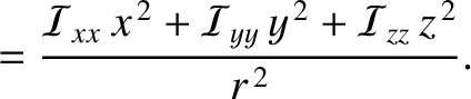
is the distribution's moment of inertia about the axis  . Thus, we deduce that
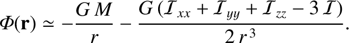 |
(8.82) |
This famous result is known as MacCullagh's formula, after its discoverer, the Irish mathematician James MacCullagh (1809–1847).
Actually,
Hence, MacCullagh's formula can also be written in the alternative form
 |
(8.84) |
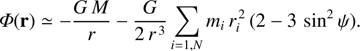
Finally, for an axisymmetric distribution, such that
 and
and
 , MacCullagh's formula reduces to
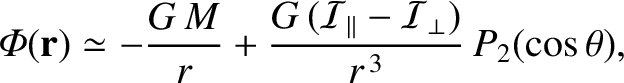 |
(8.85) |
where
 .
Of course, this expression is the same as Equation (8.69), which justifies our earlier assertion that this equation is
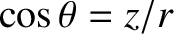
is valid for a general axisymmetric mass distribution. Incidentally, a comparison of the preceding expression with
Equation (3.66) reveals that
.
Of course, this expression is the same as Equation (8.69), which justifies our earlier assertion that this equation is
is valid for a general axisymmetric mass distribution. Incidentally, a comparison of the preceding expression with
Equation (3.66) reveals that
 |
(8.86) |
where  is the mean radius of the distribution, and the dimensionless parameter
  characterizes the
quadrupole gravitational field external to the distribution.
characterizes the
quadrupole gravitational field external to the distribution.


![\includegraphics[height=2.25in]{Chapter07/fig7_03.eps}](img1675.png)