Next: Gravitational potential energy Up: Newtonian gravity Previous: Introduction
 and
and  , located at position vectors
 and
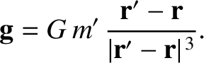
and  , respectively. According to the preceding analysis,
the acceleration
, respectively. According to the preceding analysis,
the acceleration  of mass as a result of the gravitational force exerted on it by mass takes the form
 |
(3.3) |
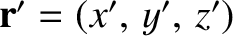
 -component of this acceleration is written
![$\displaystyle g_x = G\,m'\,\frac{x'-x}{[(x'-x)^2+(y'-y)^2+(z'-z)^2]^{\,3/2}},$](img349.png) |
(3.4) |
 and
and
 .
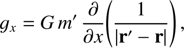
However, as is
easily demonstrated,
.
However, as is
easily demonstrated,
![$\displaystyle \frac{x'-x}{[(x'-x)^2+(y'-y)^2+(z'-z)^2]^{\,3/2}}\equiv
\frac{\partial}{\partial x}\!\left(\frac{1}{[(x'-x)^2+(y'-y)^2+(z'-z)^2]^{\,1/2}}\right).$](img352.png) |
||
| (3.5) |
 |
(3.6) |
 and
and  . It follows that
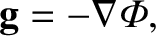
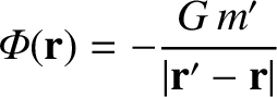
where
is termed the gravitational potential. Of course,
we can write in the form of Equation (3.7) only because gravity
is a conservative force. (See Section 2.4.)
. It follows that
where
is termed the gravitational potential. Of course,
we can write in the form of Equation (3.7) only because gravity
is a conservative force. (See Section 2.4.)
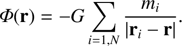
It is well known that gravity is a superposable force. In other
words, the gravitational force exerted on some point mass by a collection
of other point masses is simply the vector sum of the forces exerted on the former mass
by each of the latter masses taken in isolation. It follows that
the gravitational potential generated by a collection of point masses
at a certain location in space is the sum of the potentials generated at that
location by each point mass taken in isolation. Hence, using Equation (3.8), if there are  point masses,
  (for
(for  ), located at position vectors
  ,
then the gravitational potential generated at position vector is simply
,
then the gravitational potential generated at position vector is simply
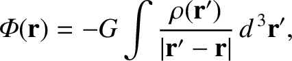
Suppose, finally, that, instead of having a collection of point masses, we have
a continuous mass distribution. In other words, let the mass at position
vector be
 , where
 is the local mass density, and
 a volume element.
Summing over all space, and taking the limit
a volume element.
Summing over all space, and taking the limit
 , we find that
Equation (3.9) yields
, we find that
Equation (3.9) yields
 , generated by
a continuous mass distribution,
, generated by
a continuous mass distribution,
 .
.