As before, we discretize in time on the uniform grid
![]() , for
, for
![]() .
Furthermore, in the
.
Furthermore, in the ![]() -direction, we discretize on the uniform grid
-direction, we discretize on the uniform grid
![]() , for
, for
![]() , where
, where
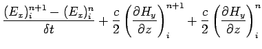
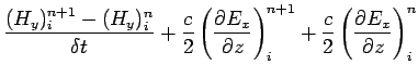
![]() . Adopting a Crank-Nicholson temporal differencing scheme
similar to that discussed in Sect. 7.4, Eqs. (253)-(254) yield
. Adopting a Crank-Nicholson temporal differencing scheme
similar to that discussed in Sect. 7.4, Eqs. (253)-(254) yield
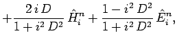
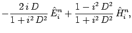
Adopting a Fourier approach, we write
 |
(259) | ||
 |
(260) |
| (261) | |||
| (262) |
Let us determine the eigenvalues ![]() of the above linear system,
assuming that
of the above linear system,
assuming that
![]() . After a little analysis,
we obtain
. After a little analysis,
we obtain
| (265) |
The routine listed below solves the 1-d wave equation using the Crank-Nicholson scheme
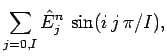
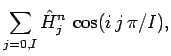
discussed above. The routine first Fourier transforms ![]() and
and ![]() , takes
a time-step using Eqs. (263) and (264), and then reconstructs
, takes
a time-step using Eqs. (263) and (264), and then reconstructs
![]() and
and ![]() via an inverse Fourier transform.
via an inverse Fourier transform.
// Wave1D.cpp
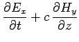
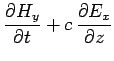
// Function to evolve 1-d wave equation:
// d E_x / dt + c d H_y / dz = 0
// d H_y / dt + c d E_x / dz = 0
// in region 0 < z < L.
// Boundary conditions:
// E_x(0,t) = E_x(L,t) = 0
// d H_y(0,t) / dz = d H_y(L,t) / dz = 0
// Arrays Ex, Hy assumed to be of extent I+1.
// Now, ith elements of arrays correspond to
// z_i = i * L / J i=0,I
// Also, D = pi c dt / (2 L), where dt is time-step.
// Uses Crank-Nicholson scheme.
#include <blitz/array.h>
using namespace blitz;
void fft_forward_cos (Array<double,1> f, Array<double,1>& F);
void fft_backward_cos (Array<double,1> F, Array<double,1>& f);
void fft_forward_sin (Array<double,1> f, Array<double,1>& F);
void fft_backward_sin (Array<double,1> F, Array<double,1>& f);
void Wave1D (Array<double,1>& Ex, Array<double,1>& Hy, double D)
{
// Find I. Declare local arrays
int I = Ex.extent(0) - 1;
Array<double,1> EE(I+1), HH(I+1), EE0(I+1), HH0(I+1);
// Fourier transform Ex and Hy
fft_forward_sin (Ex, EE0);
fft_forward_cos (Hy, HH0);
// Evolve EE and HH
for (int i = 0; i <= I; i++)
{
double x = double (i) * D;
double fp = 1. + x*x;
double fm = 1. - x*x;
EE(i) = 2. * x * HH0(i) + fm * EE0(i);
EE(i) /= fp;
HH(i) = - 2. * x * EE0(i) + fm * HH0(i);
HH(i) /= fp;
}
// Reconstruct Ex and Hy via inverse Fourier transform
fft_backward_sin (EE, Ex);
fft_backward_cos (HH, Hy);
}
Figure 230 shows an example calculation which uses the above routine to
propagate a Gaussian wave-pulse. The initial condition is
| (266) |
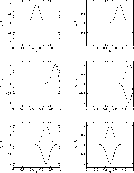 |
Figure 253 shows a second example calculation performed with the
same parameters as the first. In this calculation, the pulse is allowed to reflect
off the conducting walls ten times before returning to its initial position. Note
that the pulse amplitude and shape remain constant to a very good approximation during
this process. The fact that the pulse returns almost exactly to its initial position
after ten time periods have elapsed (i.e., at ![]() )
demonstrates that it is propagating at the
correct speed (i.e.,
)
demonstrates that it is propagating at the
correct speed (i.e., ![]() ).
).
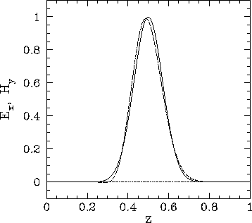 |
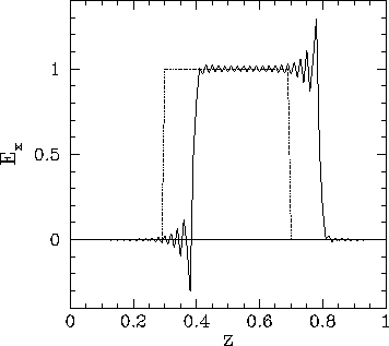
Figure 82 shows a third example calculation which uses the above listed routine to
propagate a square wave-pulse. Note that the routine does a very poor job, since
spurious oscillations are generated at the sharp leading and trailing edges of
the wave-form. As discussed in Sect. 7.5, such oscillations can
only be suppressed by adopting an upwind differencing scheme, which in this
case means that the spatial differences must be skewed in the direction from
which the wave is propagating. Unfortunately, simple explicit upwind schemes are
subject to the CFL constraint,
| (267) |
 |