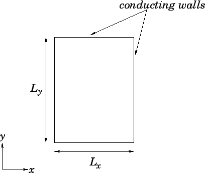
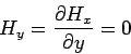
The electric and magnetic fields within the cavity can be written
![]()
![]() , and
, and
![]() , respectively.
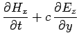
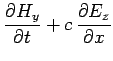
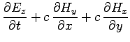
It follows from Maxwell's equations that
, respectively.
It follows from Maxwell's equations that
| (272) |
| (274) |
As usual, we discretize in time on the uniform grid
![]() , for
, for
![]() .
Furthermore, in the
.
Furthermore, in the ![]() -direction, we discretize on the uniform grid
-direction, we discretize on the uniform grid
![]() , for
, for
![]() , where
, where
![]() .
Finally, in the
.
Finally, in the ![]() -direction, we discretize on the uniform grid
-direction, we discretize on the uniform grid
![]() , for
, for
![]() , where
, where
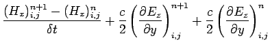
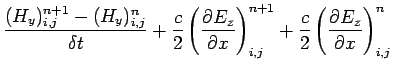
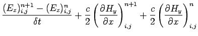
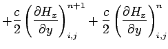
![]() . Adopting a Crank-Nicholson temporal differencing scheme
similar to that discussed in Sects. 7.4 and 7.6, Eqs. (268)-(270) yield
. Adopting a Crank-Nicholson temporal differencing scheme
similar to that discussed in Sects. 7.4 and 7.6, Eqs. (268)-(270) yield
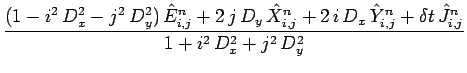
Adopting a Fourier approach, we write
 |
(278) | ||
 |
(279) | ||
 |
(280) | ||
 |
(281) |
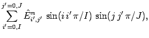
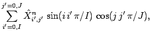
| (282) | |||
| (283) | |||
| (284) |
The routine listed below solves the 2-d wave equation in a resonant
cavity using the Crank-Nicholson scheme
discussed above. The routine first Fourier transforms ![]() ,
, ![]() ,
, ![]() , and
, and
![]() in both the
in both the ![]() - and
- and ![]() -directions, takes
a time-step using Eqs. (285)-(287), and then reconstructs
-directions, takes
a time-step using Eqs. (285)-(287), and then reconstructs
![]() ,
, ![]() , and
, and ![]() via an double inverse Fourier transform.
via an double inverse Fourier transform.
// Wave2D.cpp

// Function to evolve 2-d wave equation:

//  d H_x / dt + c d E_z / dy = 0

//  d H_y / dt + c d E_z / dx = 0

//  d E_z / dt + c d H_y / dx + c d H_x / dy = J_z

// in region 0 < x < L_x and 0 < y < L_y

// Boundary conditions:

//  E_z(0, y) = E_z(L_x, y) = E_z(x, 0) = E_z(x, L_y) = 0

//  H_x(0, y) = H_x(L_x, y) = d H_y(0, y) / dx =  d H_y(L_x, y) / dx = 0

//  H_y(x, 0) = H_y(x, L_y) = d H_x(x, 0) / dy =  d H_x(x, L_y) / dy = 0

// Matrices Hx, Hy, Ez, Jz assumed to be of extent I+1, J+1.
// Now, (i,j)th elements of matrices correspond to

//  x_i = i * dx    i=0,I

//  y_j = j * dy    j=0,J

// Here, dx = L_x / I is grid spacing in x-direction,

// and dy = L_y / J is grid spacing in x-direction.

// Now, Dx = pi c dt / (2 L_x) and Dy = pi c dt / (2 L_y),

// where dt is time-step.

// Uses Crank-Nicholson scheme.

#include <blitz/array.h>

using namespace blitz;

void fft_forward_cos (Array<double,1> f, Array<double,1>& F);
void fft_backward_cos (Array<double,1> F, Array<double,1>& f);
void fft_forward_sin (Array<double,1> f, Array<double,1>& F);
void fft_backward_sin (Array<double,1> F, Array<double,1>& f);

void Wave2D (Array<double,2>& Hx, Array<double,2>& Hy, Array<double,2>& Ez,
             Array<double,2> Jz, double Dx, double Dy, double dt)
{
  // Find I and J. Declare local arrays
  int I = Hx.extent(0) - 1;
  int J = Hx.extent(1) - 1;
  Array<double,2> X(I+1, J+1), XX(I+1, J+1), XXX(I+1, J+1);
  Array<double,2> Y(I+1, J+1), YY(I+1, J+1), YYY(I+1, J+1);
  Array<double,2> E(I+1, J+1), EE(I+1, J+1), EEE(I+1, J+1);
  Array<double,2> K(I+1, J+1), KK(I+1, J+1);

  // Fourier transform solution in x-direction
  for (int j = 0; j <= J; j++)
    {
      Array<double,1> In(I+1), Out(I+1);

      // Fourier transform Hx
      for (int i = 0; i <= I; i++) In(i) = Hx(i, j);
      fft_forward_sin (In, Out);
      for (int i = 0; i <= I; i++) X(i, j) = Out(i);

      // Fourier transform Hy
      for (int i = 0; i <= I; i++) In(i) = Hy(i, j);
      fft_forward_cos (In, Out);
      for (int i = 0; i <= I; i++) Y(i, j) = Out(i);

      // Fourier transform Ez
      for (int i = 0; i <= I; i++) In(i) = Ez(i, j);
      fft_forward_sin (In, Out);
      for (int i = 0; i <= I; i++) E(i, j) = Out(i);

      // Fourier transform Jz
      for (int i = 0; i <= I; i++) In(i) = dt * Jz(i, j);
      fft_forward_sin (In, Out);
      for (int i = 0; i <= I; i++) K(i, j) = Out(i);
    }

  // Fourier transform solution in y-direction
  for (int i = 0; i <= I; i++)
    {
      Array<double,1> In(J+1), Out(J+1);

      // Fourier transform Hx
      for (int j = 0; j <= J; j++) In(j) = X(i, j);
      fft_forward_cos (In, Out);
      for (int j = 0; j <= J; j++) XX(i, j) = Out(j);

      // Fourier transform Hy
      for (int j = 0; j <= J; j++) In(j) = Y(i, j);
      fft_forward_sin (In, Out);
      for (int j = 0; j <= J; j++) YY(i, j) = Out(j);

      // Fourier transform Ez
      for (int j = 0; j <= J; j++) In(j) = E(i, j);
      fft_forward_sin (In, Out);
      for (int j = 0; j <= J; j++) EE(i, j) = Out(j);

      // Fourier transform Jz
      for (int j = 0; j <= J; j++) In(j) = K(i, j);
      fft_forward_sin (In, Out);
      for (int j = 0; j <= J; j++) KK(i, j) = Out(j);
    }

  // Evolve XX, YY, and EE
  for (int i = 0; i <= I; i++)
    for (int j = 0; j <= J; j++)
      {
        double x = double (i) * Dx;
        double y = double (j) * Dy;
        double fp = 1. + x*x + y*y;
        double fm = 1. - x*x - y*y;

        EEE(i, j) = fm * EE(i, j) + 2. * y * XX(i, j) +
          2. * x * YY(i,j) + KK(i, j);
        EEE(i, j) /= fp;
        XXX(i, j) = XX(i, j) - y * (EEE(i, j) + EE(i, j));
        YYY(i, j) = YY(i, j) - x * (EEE(i, j) + EE(i, j));
      }

  // Reconstruct solution via inverse Fourier transform in y-direction
  for (int i = 0; i <= I; i++)
    {
      Array<double,1> In(J+1), Out(J+1);

      // Reconstruct Hx
      for (int j = 0; j <= J; j++) In(j) = XXX(i, j);
      fft_backward_cos (In, Out);
      for (int j = 0; j <= J; j++) X(i, j) = Out(j);

      // Reconstruct Hy
      for (int j = 0; j <= J; j++) In(j) = YYY(i, j);
      fft_backward_sin (In, Out);
      for (int j = 0; j <= J; j++) Y(i, j) = Out(j);

      // Reconstruct Ez
      for (int j = 0; j <= J; j++) In(j) = EEE(i, j);
      fft_backward_sin (In, Out);
      for (int j = 0; j <= J; j++) E(i, j) = Out(j);
    }

  // Reconstruct solution via inverse Fourier transform in x-direction
  for (int j = 0; j <= J; j++)
    {
      Array<double,1> In(I+1), Out(I+1);

      // Reconstruct Hx
      for (int i = 0; i <= I; i++) In(i) = X(i, j);
      fft_backward_sin (In, Out);
      for (int i = 0; i <= I; i++) Hx(i, j) = Out(i);

      // Reconstruct Hy
      for (int i = 0; i <= I; i++) In(i) = Y(i, j);
      fft_backward_cos (In, Out);
      for (int i = 0; i <= I; i++) Hy(i, j) = Out(i);

      // Reconstruct Ez
      for (int i = 0; i <= I; i++) In(i) = E(i, j);
      fft_backward_sin (In, Out);
      for (int i = 0; i <= I; i++) Ez(i, j) = Out(i);
    }
}
The numerical calculations discussed below were performed
using the above routine. The electromagnetic
fields ![]() ,
, ![]() , and
, and ![]() were all initialized to zero everywhere at
were all initialized to zero everywhere at ![]() .
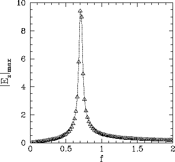
Figure 84 shows the maximum
amplitude of
.
Figure 84 shows the maximum
amplitude of ![]() versus the frequency,
versus the frequency, ![]() , for an
, for an ![]() driving
current distribution. It can
be seen that there is a clear resonance at
driving
current distribution. It can
be seen that there is a clear resonance at ![]() .
.
 |
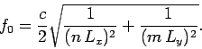
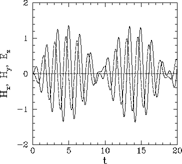
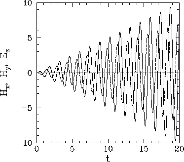
Figures 85 and 86 illustrate the typical time variation
of ![]() ,
, ![]() , and
, and ![]() for a non-resonant and a resonant case, respectively.
For the non-resonant case, the traces take the form of interference patterns
between the directly driven response, which oscillates at the driving frequency
for a non-resonant and a resonant case, respectively.
For the non-resonant case, the traces take the form of interference patterns
between the directly driven response, which oscillates at the driving frequency ![]() ,
and the transient response, which oscillates at the natural frequency
,
and the transient response, which oscillates at the natural frequency ![]() of the cavity.
Note that the transients never decay, since there is no dissipation in the present problem.
Incidentally, it is easily demonstrated that
of the cavity.
Note that the transients never decay, since there is no dissipation in the present problem.
Incidentally, it is easily demonstrated that
 |
(288) |
 |
 |
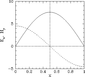
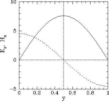
Finally, Figs. 86 and 87 illustrate the spatial
variation of the electromagnetic fields driven within the cavity when
![]() and
and ![]() .
.
 |
 |