Transmission Lines
In Sections 1.4, 2.4, and 2.6, we examined simple alternating current (ac) circuits consisting of
a single loop. In analyzing these circuits, we made the assumption that the current oscillations were in phase with one another at all points on the loop. In other words, the current passes through zero, and attains maximum/minimum
values, simultaneously at all points on the loop. Let us now consider under which circumstances this single-phase assumption
is justified. Let the current oscillate at the frequency  (in hertz), and let
  be the typical spatial extent of the
circuit. Information is presumably carried around the circuit via electromagnetic fields, which cannot
transmit information faster than the velocity of light in vacuum,
be the typical spatial extent of the
circuit. Information is presumably carried around the circuit via electromagnetic fields, which cannot
transmit information faster than the velocity of light in vacuum,  . Hence, it is only possible for the current
oscillations around the circuit to be synchronized with one another if the time required for information to propagate
around the circuit,
. Hence, it is only possible for the current
oscillations around the circuit to be synchronized with one another if the time required for information to propagate
around the circuit,  , is much less than the period of the oscillation,
  . Thus, for a given oscillation frequency,
there is a maximum circuit size,
. Thus, for a given oscillation frequency,
there is a maximum circuit size,  , above which synchronization is not possible, and the phase of the
current oscillations presumably starts to vary around the circuit. Of course,
, above which synchronization is not possible, and the phase of the
current oscillations presumably starts to vary around the circuit. Of course,
 , where
  is the
free-space wavelength of an electromagnetic wave of frequency . Hence, we deduce that the single-phase assumption breaks down when the size of an ac circuit exceeds the free-space wavelength of an electromagnetic
wave that oscillates at the alternation frequency.
is the
free-space wavelength of an electromagnetic wave of frequency . Hence, we deduce that the single-phase assumption breaks down when the size of an ac circuit exceeds the free-space wavelength of an electromagnetic
wave that oscillates at the alternation frequency.
For the case of a standard “mains” circuit, which oscillates at 60 Hz (in the US), we find that
 .
Hence, we deduce that the single-phase assumption is reasonable for such circuits. For the
case of a telephone circuit, which typically oscillates at 10 kHz (i.e., the typical frequency of human speech), we find that
.
Hence, we deduce that the single-phase assumption is reasonable for such circuits. For the
case of a telephone circuit, which typically oscillates at 10 kHz (i.e., the typical frequency of human speech), we find that
 . Thus, the single-phase assumption definitely breaks down for long-distance
telephone lines. For the case of internet cables, which typically oscillate at 10 MHz, we find that
. Thus, the single-phase assumption definitely breaks down for long-distance
telephone lines. For the case of internet cables, which typically oscillate at 10 MHz, we find that
 .
Hence, the single-phase assumption is not valid in most internet networks. Finally, for the case of TV circuits,
which typically oscillate at 10 GHz, we find that
.
Hence, the single-phase assumption is not valid in most internet networks. Finally, for the case of TV circuits,
which typically oscillate at 10 GHz, we find that
 . Thus, the single-phase
approximation breaks down completely in TV circuits. Roughly speaking, the single-phase approximation is
unlikely to hold in the type of electrical circuits involved in communication, because these invariably
require high-frequency signals to be transmitted over large distances.
. Thus, the single-phase
approximation breaks down completely in TV circuits. Roughly speaking, the single-phase approximation is
unlikely to hold in the type of electrical circuits involved in communication, because these invariably
require high-frequency signals to be transmitted over large distances.
Figure 6.1:
A section of a transmission line.
|
|
A so-called transmission line is typically used to carry high-frequency electromagnetic
signals over long distances; that is, distances sufficiently large that the
phase of the signal varies significantly along the line (which implies that the line is much longer than the
free-space wavelength of the signal).
In its simplest form, a transmission line consists of two parallel conductors
that carry equal and opposite electrical currents,  , where
  measures
distance along the line. See Figure 6.1. (This combination of two conductors carrying equal and
opposite currents is necessary to prevent intolerable losses due to electromagnetic radiation.) Let
measures
distance along the line. See Figure 6.1. (This combination of two conductors carrying equal and
opposite currents is necessary to prevent intolerable losses due to electromagnetic radiation.) Let  be the instantaneous voltage difference between the two
conductors at position . Consider a small section of the line lying
between and
be the instantaneous voltage difference between the two
conductors at position . Consider a small section of the line lying
between and
 .
If
.
If  is the electric charge on one of the conducting sections, and
  the charge on the other, then charge
conservation implies that
the charge on the other, then charge
conservation implies that
 . However, according to
standard electrical circuit theory (Fitzpatrick 2008),
. However, according to
standard electrical circuit theory (Fitzpatrick 2008),
 , where
  is the capacitance per unit length
of the line. Standard circuit theory also yields
is the capacitance per unit length
of the line. Standard circuit theory also yields
 (ibid.), where
 is the inductance per unit length of the line.
Taking the limit
is the inductance per unit length of the line.
Taking the limit
 , we obtain
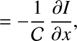
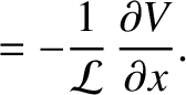
the so-called Telegrapher's equations (ibid.),
, we obtain
the so-called Telegrapher's equations (ibid.),
(See Exercise 7.)
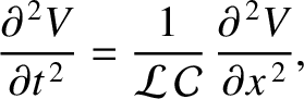
These two equations can be combined to give
 |
(6.55) |
together with an analogous equation for  .
In other words, and both
obey a wave equation of the form (6.23) in which the associated phase velocity
is
.
In other words, and both
obey a wave equation of the form (6.23) in which the associated phase velocity
is
 |
(6.56) |
Multiplying (6.53) by
 , (6.54)
by
, (6.54)
by
 , and then adding the two resulting expressions, we obtain the
energy conservation equation
, and then adding the two resulting expressions, we obtain the
energy conservation equation
 |
(6.57) |
where
 |
(6.58) |
is the electromagnetic energy density (i.e., energy per unit length) of the line, and
 |
(6.59) |
is the electromagnetic energy flux along the line (i.e., the energy per unit time that passes a given point) in the positive
-direction (ibid.).
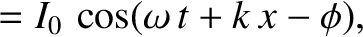
Consider a signal propagating along the line, in the positive -direction, whose associated current
takes the form
 |
(6.60) |
where  and
and  are related according to the dispersion relation
 |
(6.61) |
It can be demonstrated, from Equation (6.53), that the corresponding voltage is
 |
(6.62) |
where
 |
(6.63) |
Here,
 |
(6.64) |
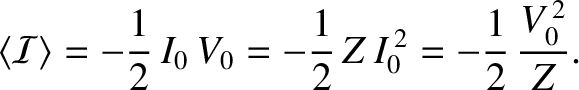
is the characteristic impedance of the line, and has units of ohms. It follows that the mean energy flux associated
with the signal is written
 |
(6.65) |
Likewise, for a signal propagating along the line in the negative
-direction,
and
the mean energy flux is
 |
(6.68) |
As a specific example, consider a transmission line consisting of two uniform parallel conducting
strips of width  and perpendicular distance apart
  , where
  . It can be demonstrated, using standard electrostatic theory (Grant and Philips 1975), that the capacitance
per unit length of the line is
. It can be demonstrated, using standard electrostatic theory (Grant and Philips 1975), that the capacitance
per unit length of the line is
 |
(6.69) |
where
 is the electric permittivity of free space.
Likewise, according to standard magnetostatic theory (ibid.), the line's inductance per
unit length takes the form
is the electric permittivity of free space.
Likewise, according to standard magnetostatic theory (ibid.), the line's inductance per
unit length takes the form
 |
(6.70) |
where
 is the magnetic
permeability of free space.
Thus, the phase velocity of a signal propagating down the line is
is the magnetic
permeability of free space.
Thus, the phase velocity of a signal propagating down the line is
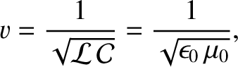 |
(6.71) |
which, of course, is the velocity of light in vacuum. [See Equation (6.120).] This is not
a coincidence. In fact, it can be demonstrated that the inductance per unit length and the capacitance per unit length of any (vacuum-filled) transmission line
satisfy (Jackson 1975)
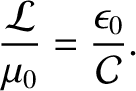 |
(6.72) |
Hence, signals always propagate down such lines at the velocity of light in vacuum.
The impedance of a parallel strip transmission line
is
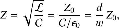 |
(6.73) |
where the quantity
 |
(6.74) |
is known as the impedance of free space. However, because we have assumed that
, it follows that the impedance of the line is impractically low (i.e.,  ). In fact, it is clear from
Exercise 11 that a signal sent down a transmission line will attenuate significantly unless the impedance of
the line greatly exceeds its resistance. Given that it is impossible to construct a practical transmission line of usable
length whose resistance is less than a few ohms, it follows that practical transmission lines must have
impedances that are much greater than an ohm (
). In fact, it is clear from
Exercise 11 that a signal sent down a transmission line will attenuate significantly unless the impedance of
the line greatly exceeds its resistance. Given that it is impossible to construct a practical transmission line of usable
length whose resistance is less than a few ohms, it follows that practical transmission lines must have
impedances that are much greater than an ohm (
 is a typical value).
Practical transmission lines generally consist of two parallel wires twisted about one another (for example, twisted-pair ethernet
cables), or two concentric cylindrical conductors (for example, co-axial TV cables). For the case of
two parallel wires of radius  and distance apart (where
  ), the capacitance per
unit length is (Wikipedia contributors 2018)
), the capacitance per
unit length is (Wikipedia contributors 2018)
 |
(6.75) |
Thus, the impedance of a parallel wire transmission line becomes
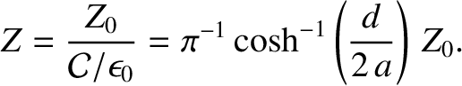 |
(6.76) |
For the case of a co-axial cable in which the radii of the inner and outer conductors are and  , respectively,
the capacitance per unit length is (Fitzpatrick 2008)
, respectively,
the capacitance per unit length is (Fitzpatrick 2008)
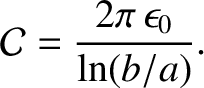 |
(6.77) |
Thus, the impedance of a co-axial transmission line becomes
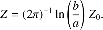 |
(6.78) |
It follows that a parallel wire transmission line of given impedance can be fabricated by choosing the appropriate ratio
of the wire spacing to the wire radius. Likewise, a co-axial transmission line of given impedance can be
fabricated by choosing the appropriate ratio of the radii of the outer and inner conductors.


![\includegraphics[width=0.6\textwidth]{Chapter06/fig6_01.eps}](img1472.png)