Energy Conservation
Consider a small-amplitude transverse wave propagating along a uniform string of infinite length, tension
 , and mass per unit length
  . (See Section 4.3.) Let
  measure
distance along the string, and let
measure
distance along the string, and let  be the transverse wave displacement.
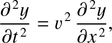
As we have seen, satisfies the wave equation
be the transverse wave displacement.
As we have seen, satisfies the wave equation
 |
(6.23) |
where
 is the phase velocity of traveling waves on the string.
Consider a section of the string lying between  and
and  . The
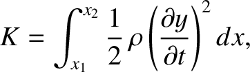
kinetic energy of this section is
. The
kinetic energy of this section is
 |
(6.24) |
because
 is the string's transverse velocity (and the longitudinal velocity is assumed to be negligibly small). The potential energy
is the work done in stretching the section, which is
is the string's transverse velocity (and the longitudinal velocity is assumed to be negligibly small). The potential energy
is the work done in stretching the section, which is
 , where
 is the difference between the section's stretched and unstretched lengths.
Here, it is assumed that the tension remains approximately constant as the
section is stretched. An element of length of the string is written
is the difference between the section's stretched and unstretched lengths.
Here, it is assumed that the tension remains approximately constant as the
section is stretched. An element of length of the string is written
![$\displaystyle ds = (dx^{\,2}+dy^{\,2})^{1/2} = \left[1+ \left(\frac{\partial y}{\partial x}\right)^2\right]^{1/2} dx.$](img1418.png) |
(6.25) |
Hence,
because it is assumed that
 (i.e., the transverse displacement is sufficiently small that the string remains
almost parallel to the -axis). Thus, the potential energy of the section is
(i.e., the transverse displacement is sufficiently small that the string remains
almost parallel to the -axis). Thus, the potential energy of the section is
 , or
, or
 |
(6.28) |
It follows that the total energy of the section is
![$\displaystyle E = \int_{x_1}^{x_2}\frac{1}{2}\left[\rho\left(\frac{\partial y}{\partial t}\right)^2
+ T\left(\frac{\partial y}{\partial x}\right)^2\right] dx.$](img1425.png) |
(6.29) |
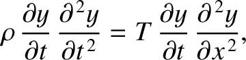
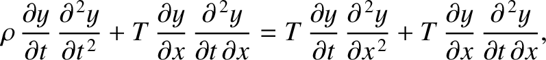
Multiplying the wave equation, (6.23), by
 ,
we obtain
,
we obtain
 |
(6.30) |
because
 .
This expression yields
.
This expression yields
 |
(6.31) |
which can be written in the form
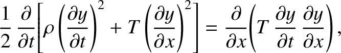 |
(6.32) |
or
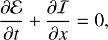 |
(6.33) |
where
![$\displaystyle {\cal E}(x,t) = \frac{1}{2}\left[\rho \left(\frac{\partial y}{\partial t}\right)^2
+ T\left(\frac{\partial y}{\partial x}\right)^2\right]$](img1432.png) |
(6.34) |
is the energy density (i.e., the energy per unit length) of the string, and
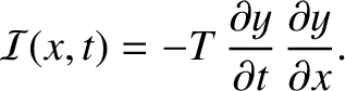 |
(6.35) |
Finally, integrating Equation (6.33) in from  to
to  , we obtain
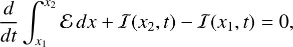 |
(6.36) |
or
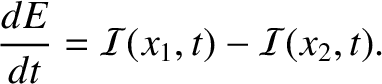 |
(6.37) |
Here,  is the energy stored in the section of the string lying between and
. [See Equation (6.29).] If we interpret
is the energy stored in the section of the string lying between and
. [See Equation (6.29).] If we interpret
 as the instantaneous energy flux (i.e., rate of energy flow)
in the positive- direction, at position and time
as the instantaneous energy flux (i.e., rate of energy flow)
in the positive- direction, at position and time  , then the previous equation
can be recognized as a declaration of energy conservation. Basically,
the equation states that the
rate of increase in the energy stored in the section of the string lying between and , which is
, then the previous equation
can be recognized as a declaration of energy conservation. Basically,
the equation states that the
rate of increase in the energy stored in the section of the string lying between and , which is  , is equal to the difference between the rate at which energy flows into
the left end of the section, which is
, is equal to the difference between the rate at which energy flows into
the left end of the section, which is
 , and the rate at which it flows out of the right end, which is
 . Incidentally, the string conserves energy
because it lacks any mechanism for energy dissipation. The same is true of the
other wave media discussed in this chapter.
. Incidentally, the string conserves energy
because it lacks any mechanism for energy dissipation. The same is true of the
other wave media discussed in this chapter.
Consider a wave propagating in the positive -direction of the form
 |
(6.38) |
According to Equation (6.35), the energy flux associated with this
wave is
 |
(6.39) |
Thus, the mean energy flux is written
 |
(6.40) |
where
 represents an average over a period of the wave oscillation. Here, use
has been made of
represents an average over a period of the wave oscillation. Here, use
has been made of
 , as well as the result that
 for all
  . Moreover, the quantity
 |
(6.41) |
is known as the characteristic impedance of the string. The units of  are force over velocity. Thus, the string impedance measures the
typical tension required to produce a unit transverse velocity.
Finally, according to Equation (6.40), a traveling wave propagating in the positive -direction
is associated with a positive energy flux. In other words, the wave transports energy
in the positive -direction.
are force over velocity. Thus, the string impedance measures the
typical tension required to produce a unit transverse velocity.
Finally, according to Equation (6.40), a traveling wave propagating in the positive -direction
is associated with a positive energy flux. In other words, the wave transports energy
in the positive -direction.
Consider a wave propagating in the negative -direction of the general form
 |
(6.42) |
It can be demonstrated, from Equation (6.35), that the mean energy flux
associated with this wave is
 |
(6.43) |
The fact that the energy flux is negative means that the wave transports energy in
the negative -direction.
Suppose that we have a superposition of a wave of amplitude  propagating in the
positive -direction, and a wave of amplitude
propagating in the
positive -direction, and a wave of amplitude  propagating
in the negative -direction, so that
propagating
in the negative -direction, so that
 |
(6.44) |
According to Equation (6.35), the instantaneous energy flux is written
Hence, the mean energy flux,
 |
(6.46) |
is the difference between the independently calculated mean fluxes associated with the waves traveling
to the right (i.e., in the positive -direction) and to the left. Recall, from the previous section, that a standing wave
is a superposition of two traveling waves, of equal amplitude and frequency,
propagating in opposite directions. It immediately follows, from the previous expression,
that a standing wave has zero associated net energy flux. In other words,
a standing wave does not give rise to net energy transport.
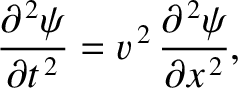
We saw earlier, in Section 5.3, that a small-amplitude longitudinal wave in
a thin elastic rod satisfies the wave equation,
 |
(6.47) |
where  is the longitudinal wave displacement,
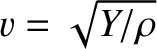 the phase velocity of traveling waves along the rod,
  the Young's modulus, and the
mass density. Using similar analysis to that just employed,
we can derive an energy conservation equation of the form (6.33) from this
wave equation, where
the Young's modulus, and the
mass density. Using similar analysis to that just employed,
we can derive an energy conservation equation of the form (6.33) from this
wave equation, where
![$\displaystyle {\cal E} = \frac{1}{2}\left[\rho\left(\frac{\partial\psi}{\partial t}\right)^2 + Y\left(\frac{\partial \psi}{\partial x}\right)^2\right]$](img1459.png) |
(6.48) |
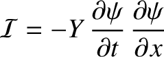
is the wave energy density (i.e., the energy per unit volume), and
 |
(6.49) |
the wave energy flux (i.e., the rate of energy flow per unit area) in the positive -direction.
For a traveling wave of the form
 , the
previous expression yields
, the
previous expression yields
|
(6.50) |
where
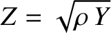 |
(6.51) |
is the impedance of the rod. The units of are pressure over velocity. Hence, in this
case, the
impedance measures the typical pressure in the rod required to produce a
unit longitudinal velocity.
Analogous arguments reveal that the impedance
of an ideal gas of density , pressure  , and ratio of specific heats
  ,
is
,
is
 |
(6.52) |
(See Section 5.4.)

![$\displaystyle = \int_{x_1}^{x_2} \left\{\left[1+ \left(\frac{\partial y}{\partial x}\right)^2\right]^{1/2}-1\right\} dx$](img1420.png)
![$\displaystyle \omega^{\,2}\,Z\left[A_+\,\sin(\omega\,t-k\,x-\phi_+)+A_-\,\sin(\omega\,t+k\,x-\phi_-)\right]$](img1454.png)
![$\displaystyle \left[A_+\,\sin(\omega\,t-k\,x-\phi_+)-A_-\,\sin(\omega\,t+k\,x-\phi_-)\right]$](img1455.png)

![$\displaystyle \omega^{\,2}\,Z\left[A_+^{\,2}\,\sin^2(\omega\,t-k\,x-\phi_+) - A_-^{\,2}\,\sin^2(\omega\,t+k\,x-\phi_-)\right].$](img1456.png)