Next: Driven Damped Harmonic Oscillation Up: Damped and Driven Harmonic Previous: Quality Factor Contents
 , connected
in series with a capacitor, of capacitance
, connected
in series with a capacitor, of capacitance  , and a resistor, of resistance
  . See Figure 2.2. Such
a circuit is known as an LCR circuit, for obvious reasons. Suppose that
. See Figure 2.2. Such
a circuit is known as an LCR circuit, for obvious reasons. Suppose that
 is the instantaneous current flowing around the circuit. As we saw in Section 1.4, the potential drops across the inductor and the capacitor are
 and
and  , respectively. Here,
  is the charge on the capacitor's positive plate, and
  . Moreover, from Ohm's law, the potential drop across the resistor is
  (Fitzpatrick 2008). Kirchhoff's second circuital law states that the sum of the potential drops across the
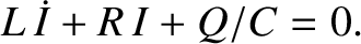
various components of a closed circuit loop is zero. It follows that
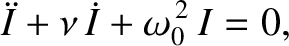
Dividing by , and differentiating with respect to time, we obtain
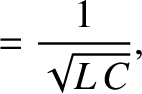
where
Comparison with Equation (2.2) reveals that Equation (2.33)
is a damped harmonic oscillator equation. Thus, provided that the
resistance is not too high (i.e., provided
(Fitzpatrick 2008). Kirchhoff's second circuital law states that the sum of the potential drops across the
various components of a closed circuit loop is zero. It follows that
Dividing by , and differentiating with respect to time, we obtain
where
Comparison with Equation (2.2) reveals that Equation (2.33)
is a damped harmonic oscillator equation. Thus, provided that the
resistance is not too high (i.e., provided
 , which is equivalent to
 ), the current
in the circuit executes damped harmonic oscillations of the form [cf., Equation (2.12)]
), the current
in the circuit executes damped harmonic oscillations of the form [cf., Equation (2.12)]
 |
(2.36) |
 and
and  are constants, and
 .
We conclude that if a small amount of resistance is introduced into an LC circuit then the characteristic oscillations in the current damp away exponentially
at a rate proportional to the resistance.
.
We conclude that if a small amount of resistance is introduced into an LC circuit then the characteristic oscillations in the current damp away exponentially
at a rate proportional to the resistance.
Multiplying Equation (2.32) by  , and making use of the fact that ,
we obtain
, and making use of the fact that ,
we obtain
 |
(2.37) |
 |
(2.39) |
 is the circuit energy; that is, the sum of the energies stored in the inductor
and the capacitor. Moreover, according to Equation (2.38), the circuit
energy decays in time due to the power
is the circuit energy; that is, the sum of the energies stored in the inductor
and the capacitor. Moreover, according to Equation (2.38), the circuit
energy decays in time due to the power
 dissipated via Joule heating in the resistor (Fitzpatrick 2008). Of course, the dissipated power is always positive. In other words, the circuit
never gains energy from the resistor.
dissipated via Joule heating in the resistor (Fitzpatrick 2008). Of course, the dissipated power is always positive. In other words, the circuit
never gains energy from the resistor.
Finally, a comparison of Equations (2.31), (2.34), and (2.35) reveals that the quality factor of an LCR circuit is
 |
(2.40) |


![\includegraphics[width=0.5\textwidth]{Chapter02/fig2_02.eps}](img503.png)