Driven Damped Harmonic Oscillation
We saw earlier, in Section 2.2, that if a damped mechanical oscillator is set into motion then the oscillations
eventually die away due to frictional energy losses. In fact, the only way of maintaining
the amplitude of a damped oscillator is to continuously feed energy into the system in such a
manner as
to offset the frictional losses. A steady (i.e., constant amplitude) oscillation of this type is called driven damped harmonic oscillation.
Consider a modified version of the mass–spring system investigated in Section 2.2 in which one end of the spring is
attached to the mass, and the other to an oscillating piston. See Figure 2.3.
Let  be the horizontal displacement of the mass, and
  the horizontal
displacement of the piston. The extension of the spring is thus
the horizontal
displacement of the piston. The extension of the spring is thus  , assuming
that the spring is unstretched when
, assuming
that the spring is unstretched when  . Thus, the horizontal force acting
on the mass can be written [cf., Equation (2.1)]
. Thus, the horizontal force acting
on the mass can be written [cf., Equation (2.1)]
 |
(2.41) |
The equation of motion of the system then becomes [cf., Equation (2.2)]
 |
(2.42) |
where  is the damping constant, and
 the undamped oscillation frequency.
Suppose, finally, that the piston executes simple harmonic oscillation of
angular frequency
the undamped oscillation frequency.
Suppose, finally, that the piston executes simple harmonic oscillation of
angular frequency  and amplitude
  , so that the time evolution
equation of the system takes the form
, so that the time evolution
equation of the system takes the form
 |
(2.43) |
We shall refer to the preceding equation as the driven damped harmonic oscillator equation.
Figure 2.3:
A driven oscillatory system.
|
|
We would generally expect the periodically driven oscillator shown in Figure 2.3 to eventually settle down to
a steady (i.e., constant amplitude) pattern of oscillation, with the same frequency as the piston, in which the frictional energy
loss per cycle is exactly matched by the work done by the piston per cycle. (See Exercise 9.) This suggests
that we should search for a solution to Equation (2.43) of the form
 |
(2.44) |
Here,  is the amplitude of the driven oscillation, whereas
  is the phase lag of this oscillation (with respect to the phase of the piston oscillation).
Because
Equation (2.43) becomes
is the phase lag of this oscillation (with respect to the phase of the piston oscillation).
Because
Equation (2.43) becomes
 |
(2.47) |
However,
 and
and
 (see Appendix B), so
we obtain
where we have collected similar terms.
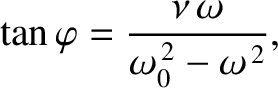
The only way in which the preceding equation can be satisfied at all times is if
the (constant) coefficients of
(see Appendix B), so
we obtain
where we have collected similar terms.
The only way in which the preceding equation can be satisfied at all times is if
the (constant) coefficients of
 and
and
 separately equate to
zero. In other words, if
These two expressions can be combined to give
This follows because Equation (2.50) yields
separately equate to
zero. In other words, if
These two expressions can be combined to give
This follows because Equation (2.50) yields
 |
(2.53) |
and so
(See Appendix B.)
Hence, substitution into Equation (2.49) gives Equation (2.51).
Figure 2.4:
Driven damped harmonic oscillation. The figure shows the relative amplitude of the motion plotted as a function of
the driving frequency for
various different values of the damping rate. In fact,
 ,
,  ,
,  ,
,  , and
, and  correspond to the solid, dotted, short-dashed, long-dashed,
and dot-dashed curves, respectively.
correspond to the solid, dotted, short-dashed, long-dashed,
and dot-dashed curves, respectively.
|
|
Let us investigate the dependence of the amplitude,  , and phase lag, , of the driven oscillation on the driving frequency,
 . This is most easily done graphically. Figures 2.4 and 2.5 show
 and plotted as functions of for
various different values of
and plotted as functions of for
various different values of
 . It can be seen that as the amount of
damping in the system is decreased the amplitude of the response becomes
progressively more peaked at the system's natural frequency of oscillation,
. It can be seen that as the amount of
damping in the system is decreased the amplitude of the response becomes
progressively more peaked at the system's natural frequency of oscillation,  . This effect is known as resonance, and
is termed the resonant frequency. Thus,
a weakly damped oscillator (i.e.,
. This effect is known as resonance, and
is termed the resonant frequency. Thus,
a weakly damped oscillator (i.e.,
 ) can be driven to large amplitude by the application of a relatively
small amplitude external driving force that oscillates at a frequency close to the resonant frequency. The response of the oscillator is in phase (i.e.,
) can be driven to large amplitude by the application of a relatively
small amplitude external driving force that oscillates at a frequency close to the resonant frequency. The response of the oscillator is in phase (i.e.,
 )
with the external drive for driving frequencies well below the resonant
frequency, is in phase quadrature
(i.e.,
)
with the external drive for driving frequencies well below the resonant
frequency, is in phase quadrature
(i.e.,
 )
at the resonant frequency, and is in anti-phase (i.e.,
)
at the resonant frequency, and is in anti-phase (i.e.,
 )
for frequencies well above the resonant frequency.
)
for frequencies well above the resonant frequency.
Figure 2.5:
Driven damped harmonic oscillation. The figure shows the relative phase of the motion plotted as a function of
the driving frequency for
various different values of the damping rate. In fact,
, , , , and correspond to the solid, dotted, short-dashed, long-dashed,
and dot-dashed curves, respectively.
|
|
According to Equations (2.31) and (2.51),
 |
(2.56) |
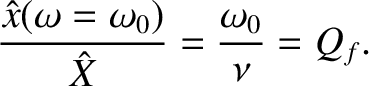
In other words, if the driving frequency matches the resonant frequency then the ratio of the amplitude of the driven oscillation
to that of the piston oscillation is equal to the quality factor,  . Hence, can be interpreted as the resonant
amplification factor of the oscillator.
Equations (2.51) and (2.55) imply that,
for a weakly damped oscillator (i.e.,
) which
is close to resonance [i.e.,
. Hence, can be interpreted as the resonant
amplification factor of the oscillator.
Equations (2.51) and (2.55) imply that,
for a weakly damped oscillator (i.e.,
) which
is close to resonance [i.e.,
 ],
],
![$\displaystyle \frac{\hat{x}(\omega)}{\hat{x}(\omega=\omega_0)}\simeq \sin\varphi\simeq \frac{\nu}{[4\,(\omega_0-\omega)^{\,2} + \nu^{\,2}]^{1/2}}.$](img552.png) |
(2.57) |
This follows because
 .
Hence, the width of the resonance
peak (in angular frequency) is
.
Hence, the width of the resonance
peak (in angular frequency) is
 , where the edges of the peak are defined as the points where the driven amplitude
is reduced to
, where the edges of the peak are defined as the points where the driven amplitude
is reduced to
 of its maximum value; that is,
 . The phase lag at the low- and high-frequency edges of the
peak are
. The phase lag at the low- and high-frequency edges of the
peak are  and
and  , respectively. Furthermore, the
fractional width of the peak is
, respectively. Furthermore, the
fractional width of the peak is
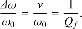 |
(2.58) |
We conclude that the
height and width of the resonance peak of a weakly damped ( ) harmonic oscillator scale as and
 , respectively. Thus, the area under the resonance peak stays
approximately constant as varies.
, respectively. Thus, the area under the resonance peak stays
approximately constant as varies.
The force exerted on the system by the piston is
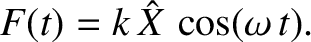 |
(2.59) |
Hence, the instantaneous power absorption from the piston becomes
The average power absorption during an oscillation cycle is
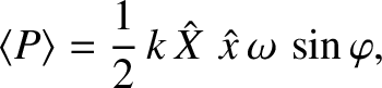 |
(2.61) |
because
 and
and
 . Given that the amplitude of the driven oscillation neither grows nor decays, the average power absorption from the piston during an oscillation cycle must equal the average power dissipation due to friction. (See Exercise 9.)
Making use of Equations (2.56) and (2.57), the mean power absorption when the driving
frequency is close to the resonant frequency is
. Given that the amplitude of the driven oscillation neither grows nor decays, the average power absorption from the piston during an oscillation cycle must equal the average power dissipation due to friction. (See Exercise 9.)
Making use of Equations (2.56) and (2.57), the mean power absorption when the driving
frequency is close to the resonant frequency is
![$\displaystyle \langle P\rangle \simeq \frac{1}{2}\,\omega_0\,k\,\hat{X}^{\,2}\,Q_f\left[\frac{\nu^{\,2}}{4\,(\omega_0-\omega)^{\,2}+\nu^{\,2}}\right].$](img569.png) |
(2.62) |
Thus, the maximum power absorption occurs at the resonance (i.e.,
 ), and the absorption is reduced to half of this maximum value at the edges of the
resonance (i.e.,
). Furthermore, the peak power
absorption is proportional to the quality factor, , which means that it is inversely
proportional to the damping constant,
), and the absorption is reduced to half of this maximum value at the edges of the
resonance (i.e.,
). Furthermore, the peak power
absorption is proportional to the quality factor, , which means that it is inversely
proportional to the damping constant,  .
.


![$\displaystyle \left[\hat{x}\left(\omega_0^{\,2}-\omega^{\,2}\right)\cos\varphi + \hat{x}\,\nu\,\omega\,\sin\varphi -\omega_0^{\,2}\,\hat{X}\right]\cos(\omega\,t)$](img526.png)
![$\displaystyle +\hat{x}\left[\left(\omega_0^{\,2}-\omega^{\,2}\right)\sin\varphi-\nu\,\omega\,\cos\varphi\right]\sin(\omega\,t)$](img527.png)


![$\displaystyle \equiv \frac{1}{\sqrt{1+\tan^2\varphi}} = \frac{\omega_0^{\,2}-\o...
...\omega_0^{\,2}-\omega^{\,2}\right)^{\,2}+\nu^{\,2}\,\omega^{\,2}\right]^{1/2}},$](img538.png)

![$\displaystyle \equiv \frac{\tan\varphi}{\sqrt{1+\tan^2\varphi}} = \frac{\nu\,\o...
...\omega_0^{\,2}-\omega^{\,2}\right)^{\,2}+\nu^{\,2}\,\omega^{\,2}\right]^{1/2}}.$](img540.png)
![\includegraphics[width=0.8\textwidth]{Chapter02/fig2_04.eps}](img541.png)
![\includegraphics[width=0.8\textwidth]{Chapter02/fig2_05.eps}](img549.png)


![$\displaystyle = -k\,\hat{X}\,\hat{x}\,\omega\left[\cos(\omega\,t)\,\sin(\omega\,t)\,\cos\varphi - \cos^2(\omega\,t)\,\sin\varphi\right].$](img565.png)
![\includegraphics[width=0.9\textwidth]{Chapter02/fig2_03.eps}](img517.png)


![$\displaystyle = \frac{\omega_0^{\,2}\,\hat{X}}{\left[\left(\omega_0^{\,2}-\omega^{\,2}\right)^{\,2}+\nu^{\,2}\,\omega^{\,2}\right]^{1/2}},$](img533.png)