


Next: Exercises
Up: Quantum Statistics
Previous: Neutron Stars
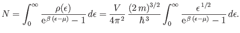
Consider a gas of weakly-interacting bosons. It is helpful to define the gas's chemical potential,
 |
(8.221) |
whose value is determined by the equation
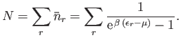 |
(8.222) |
Here,  is the total number of particles, and
 the energy of the single-particle
quantum state
the energy of the single-particle
quantum state  .
Because, in general, the energies of the quantum states are very closely spaced, the sum in the previous expression can
approximated as an integral. Now, according to Section 8.12, the number of quantum states per unit volume
with wavenumbers in the range
.
Because, in general, the energies of the quantum states are very closely spaced, the sum in the previous expression can
approximated as an integral. Now, according to Section 8.12, the number of quantum states per unit volume
with wavenumbers in the range  to
to  is
is
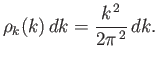 |
(8.223) |
However, the energy of a state with wavenumber
is
 |
(8.224) |
where  is the boson mass. Let
 be the number of bosons
whose energies lies in the range
be the number of bosons
whose energies lies in the range  to
to
 . It follows that
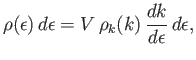 |
(8.225) |
where  is the volume of the gas.
Here, we are assuming that the bosons are spinless, so that there is only one particle state per translational state.
Hence,
is the volume of the gas.
Here, we are assuming that the bosons are spinless, so that there is only one particle state per translational state.
Hence,
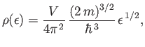 |
(8.226) |
and Equation (8.222) becomes
 |
(8.227) |
However, there is a significant flaw in this formulation. In using the integral approximation, rather than performing the sum, the ground-state,
 , has
been left out [because
, has
been left out [because  ]. Under ordinary circumstances, this omission does not matter. However, at very low temperatures, bosons tend to condense into
the ground-state, and the occupation number of this state becomes very much larger than that of any other state. Under these circumstances, the ground-state must be included
in the calculation.
]. Under ordinary circumstances, this omission does not matter. However, at very low temperatures, bosons tend to condense into
the ground-state, and the occupation number of this state becomes very much larger than that of any other state. Under these circumstances, the ground-state must be included
in the calculation.
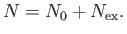
We can overcome the previous difficulty in the following manner. Let there be  bosons in the ground-state, and
 in the
various excited states, so that
in the
various excited states, so that
 |
(8.228) |
Because the ground-state is excluded from expression (8.227), the integral only gives the number of bosons in excited states.
In other words,
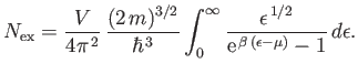 |
(8.229) |
Now, because the ground-state has zero energy, its mean occupancy number is
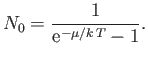 |
(8.230) |
Moreover, at temperatures very close to absolute zero, we expect
 , which implies that
 |
(8.231) |
We conclude that
 |
(8.232) |
for large
. Hence, at very low temperatures, we can safely set
 equal to unity in Equation (8.229).
Thus, we obtain
equal to unity in Equation (8.229).
Thus, we obtain
 |
(8.233) |
where
 . The value of the integral is
 , where
 is a Gamma
function, and
is a Gamma
function, and
 a Riemann zeta function. (See Exercise 4.) Furthermore,
 ,
and
,
and
 . Hence,
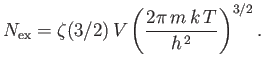 |
(8.234) |
The so-called Bose temperature,  , is defined as the temperature above which all the bosons are in excited states.
Setting
, is defined as the temperature above which all the bosons are in excited states.
Setting
 and
and  in the previous expression, we obtain
![$\displaystyle T_B = \frac{h^{ 2}}{2\pi m k}\left[\frac{N}{\zeta(3/2) V}\right]^{ 2/3}.$](img2430.png) |
(8.235) |
Moreover,
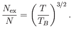 |
(8.236) |
Thus, the fractional number of bosons in the ground-state is
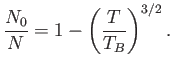 |
(8.237) |
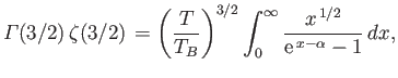
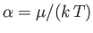
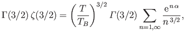
Obviously, the preceding two equations are only valid for 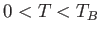 . For
. For  , we have
  and
and
 .
Moreover, for
we have
.
Moreover, for
we have
 , whereas for
, combining Equations (8.229) (with
) and (8.235)
yields
, whereas for
, combining Equations (8.229) (with
) and (8.235)
yields
 |
(8.238) |
where
and
 . Expanding in powers of
 , we obtain
 |
(8.239) |
where  (see Exercise 4), which reduces to
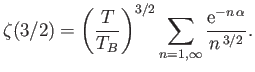 |
(8.240) |
The previous equation can be solved numerically to give
 as a function of
  .
.
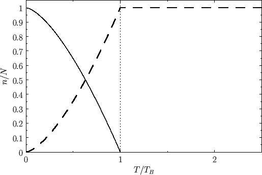
Figure:
Variation with temperature of  (solid curve) and
 (dashed curve) for a boson gas.
 |
Let us estimate a typical value of the Bose temperature. Consider a boson gas made up of
 atoms confined to a volume of 1 litre. The mass
of a
atom is
atoms confined to a volume of 1 litre. The mass
of a
atom is
 . Making use of Equation (8.235), we
obtain
. Making use of Equation (8.235), we
obtain
![$\displaystyle T_B = \frac{(6.63\times 10^{-34})^{ 2}}{2\pi (6.65\times 10^{-2...
....02\times 10^{ 22}}{(2.612) (1\times 10^{-3})}\right]^{ 2/3}=0.062 {\rm K}.$](img2449.png) |
(8.241) |
At atmospheric pressure, helium liquifies at
 , long before the Bose temperature is reached. In fact, all real gases liquify before the Bose temperature is reached.
Figure:
Variation with temperature of
 for a boson gas.
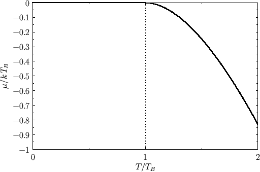 |
Figure 8.7 shows the variation of
and
with
. A corresponding graph of
[numerically determined from Equation (8.240) when
] is shown in Figure 8.8. The sudden collapse
of bosons into the ground-state at temperatures below the Bose temperature is known as Bose-Einstein condensation. In
1995, E.A. Cornell and C.E. Wieman led a team of physicists that created a nearly pure condensate by cooling a vapor of rubidium atoms to a temperature of
 . (Cornell and Wieman were subsequently awarded the Nobel prize in 2001.)
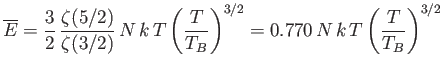
The mean energy of a boson gas takes the form
 |
(8.242) |
As before, we can approximate the sum as an integral, and write
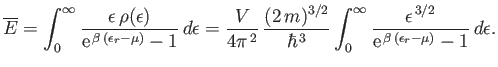 |
(8.243) |
In this case, we do not need to worry about the omission of the ground-state in the integral, because this state makes no contribution to the mean
energy (because
in the ground-state). For temperatures above the Bose temperature, all the bosons
are in excited states, and we expect the mean energy to approach the classical value,
 . However, below the
Bose temperature, a substantial fraction of bosons are in the ground-state, so we expect the mean energy to fall well below the
classical value.
. However, below the
Bose temperature, a substantial fraction of bosons are in the ground-state, so we expect the mean energy to fall well below the
classical value.
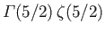
As we have seen, the chemical potential of a boson gas is very close to zero for temperatures below the Bose temperature. Hence,
setting  in the previous expression, and making the substitution
, we obtain
in the previous expression, and making the substitution
, we obtain
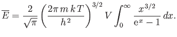 |
(8.244) |
The integral is equal to
 , where
 , and
, and
 . (See Exercise 4.)
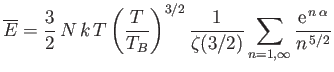
Thus, we obtain
. (See Exercise 4.)
Thus, we obtain
 |
(8.245) |
where use has been made of Equation (8.235). Note that
 for temperatures below the Bose temperature, but
that
for temperatures below the Bose temperature, but
that
 becomes similar in magnitude to the classical value,
, as
becomes similar in magnitude to the classical value,
, as
 . The molar specific heat below the Bose temperature is
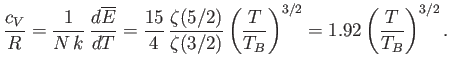 |
(8.246) |
Likewise, the mean pressure is
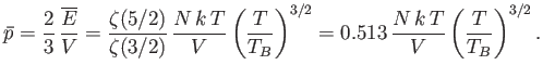 |
(8.247) |
(See Exercise 7.) In both cases, the quantities become similar in magnitude to their classical values as
, but
fall far below these values when  .
.
Figure:
Variation with temperature of
 for a boson gas, where
 .
.
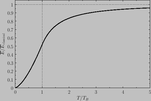 |
For
, Equation (8.243) becomes
 |
(8.248) |
(see Exercise 4), where  is determined from the numerical solution of Equation (8.240). Figure 8.9 shows how
the mean energy of a boson gas varies with temperature, and clearly illustrates that the energy approaches
its classical value asymptotically in the limit
is determined from the numerical solution of Equation (8.240). Figure 8.9 shows how
the mean energy of a boson gas varies with temperature, and clearly illustrates that the energy approaches
its classical value asymptotically in the limit  . Finally, Figure 8.10 shows how the molar heat capacity of a boson gas
varies with temperature. It can be seen that the
. Finally, Figure 8.10 shows how the molar heat capacity of a boson gas
varies with temperature. It can be seen that the  curve has a change in slope at
, reaching a maximum value there of
curve has a change in slope at
, reaching a maximum value there of
 . At higher temperatures,
approaches the classical value,
. At higher temperatures,
approaches the classical value,  , asymptotically.
Figure:
Variation with temperature of
 for a boson gas, where
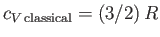 .
.
 |
Next: Exercises
Up: Quantum Statistics
Previous: Neutron Stars
Richard Fitzpatrick
2016-01-25