Next: Hydrogen Atom
Up: Central Potentials
Previous: Derivation of Radial Equation
Infinite Spherical Potential Well
Consider a particle of mass  and energy
  moving in the
following simple central potential:
moving in the
following simple central potential:
![\begin{displaymath}
V(r) = \left\{\begin{array}{lcl}
0&\mbox{\hspace{1cm}}&\mbox...
...leq a$}\ [0.5ex]
\infty&&\mbox{otherwise}
\end{array}\right..
\end{displaymath}](img1537.png) |
(647) |
Clearly, the wavefunction  is only non-zero in the region
 .
Within this region, it is subject to the physical boundary conditions that it be well behaved (i.e.,
square-integrable) at
.
Within this region, it is subject to the physical boundary conditions that it be well behaved (i.e.,
square-integrable) at  , and that it be zero at
  (see Sect. 5.2).
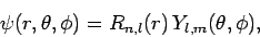
Writing the wavefunction in the standard form
(see Sect. 5.2).
Writing the wavefunction in the standard form
 |
(648) |
we deduce (see previous section) that the radial function  satisfies
 |
(649) |
in the region
, where
 |
(650) |
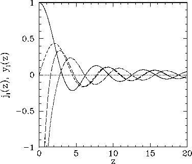
Figure 20:
The first few spherical Bessel functions. The solid, short-dashed, long-dashed, and dot-dashed curves show  ,
,  ,
,  , and
, and  , respectively.
 |
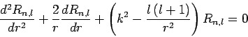
Defining the scaled radial variable  , the above differential
equation can be transformed into the standard form
, the above differential
equation can be transformed into the standard form
![\begin{displaymath}
\frac{d^2 R_{n,l}}{dz^2} + \frac{2}{z}\frac{dR_{n,l}}{dz} + \left[1
- \frac{l (l+1)}{z^2}\right] R_{n,l} = 0.
\end{displaymath}](img1546.png) |
(651) |
The two independent solutions to this well-known second-order differential equation are called spherical Bessel
functions,![[*]](footnote.png) and can be written
and can be written
Thus, the first few spherical Bessel functions take the form
These functions are also plotted in Fig. 20. It can be seen that
the spherical Bessel functions are oscillatory in nature, passing through
zero many times. However, the  functions are badly
behaved (i.e., they are not square-integrable) at
functions are badly
behaved (i.e., they are not square-integrable) at  , whereas
the
, whereas
the  functions are well behaved everywhere. It follows from
our boundary condition at that the are unphysical, and that the radial wavefunction
is thus proportional to
functions are well behaved everywhere. It follows from
our boundary condition at that the are unphysical, and that the radial wavefunction
is thus proportional to  only. In order to satisfy the boundary
condition at [i.e.,
only. In order to satisfy the boundary
condition at [i.e.,  ], the value of
  must
be chosen such that
must
be chosen such that  corresponds to one of the zeros of .
Let us denote the
corresponds to one of the zeros of .
Let us denote the  th zero of as
  . It follows that
 |
(658) |
for
 .
Hence, from (650), the allowed energy levels are
.
Hence, from (650), the allowed energy levels are
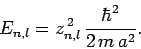 |
(659) |
The first few values of are listed in Table 1. It
can be seen that is an increasing function of both and  .
.
Table 1:
The first few zeros of the spherical Bessel function .
| |
 |
 |
 |
 |
 |
3.142 |
6.283 |
9.425 |
12.566 |
 |
4.493 |
7.725 |
10.904 |
14.066 |
 |
5.763 |
9.095 |
12.323 |
15.515 |
 |
6.988 |
10.417 |
13.698 |
16.924 |
 |
8.183 |
11.705 |
15.040 |
18.301 |
|
We are now in a position to interpret the three quantum numbers--, ,
and --which determine the form of the wavefunction
specified in Eq. (648). As is clear from Sect. 8, the
azimuthal quantum number determines the number of nodes in the
wavefunction as the azimuthal angle  varies between 0 and
  . Thus,
  corresponds to no nodes,
  to a single node,
  to two nodes,
etc. Likewise, the polar quantum number determines the
number of nodes in the wavefunction as the polar angle
to two nodes,
etc. Likewise, the polar quantum number determines the
number of nodes in the wavefunction as the polar angle  varies between 0 and
  .
Again, corresponds to no nodes, to a single node,
etc. Finally, the radial quantum number determines
the number of nodes in the wavefunction as the radial
variable
.
Again, corresponds to no nodes, to a single node,
etc. Finally, the radial quantum number determines
the number of nodes in the wavefunction as the radial
variable  varies between 0 and
  (not counting any
nodes at or ). Thus, corresponds to no nodes,
to a single node, to two nodes, etc. Note that,
for the
case of an infinite potential well,
the only restrictions on the values that the various quantum numbers can take are that must be a positive integer, must be
a non-negative integer, and must be an integer lying between
(not counting any
nodes at or ). Thus, corresponds to no nodes,
to a single node, to two nodes, etc. Note that,
for the
case of an infinite potential well,
the only restrictions on the values that the various quantum numbers can take are that must be a positive integer, must be
a non-negative integer, and must be an integer lying between  and . Note, further,
that the allowed energy levels (659) only depend on the
values of the quantum numbers and . Finally, it is
easily demonstrated that the spherical Bessel functions are mutually
orthogonal: i.e.,
and . Note, further,
that the allowed energy levels (659) only depend on the
values of the quantum numbers and . Finally, it is
easily demonstrated that the spherical Bessel functions are mutually
orthogonal: i.e.,
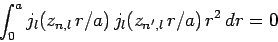 |
(660) |
when  .
Given that the
.
Given that the
 are mutually orthogonal (see Sect. 8), this ensures that wavefunctions (648) corresponding to distinct
sets of values of the quantum numbers , , and are mutually
orthogonal.
are mutually orthogonal (see Sect. 8), this ensures that wavefunctions (648) corresponding to distinct
sets of values of the quantum numbers , , and are mutually
orthogonal.
Next: Hydrogen Atom
Up: Central Potentials
Previous: Derivation of Radial Equation
Richard Fitzpatrick
2010-07-20