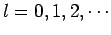
Next: Determination of Phase-Shifts
Up: Scattering Theory
Previous: Born Approximation
We can assume, without loss of generality, that the incident wavefunction
is characterized by a wavevector  which is aligned parallel to the
  -axis.
The scattered wavefunction is characterized by a wavevector
-axis.
The scattered wavefunction is characterized by a wavevector  which has the same magnitude as , but, in general, points
in a different direction. The direction of is specified
by the polar angle
which has the same magnitude as , but, in general, points
in a different direction. The direction of is specified
by the polar angle  (i.e., the angle subtended between the
two wavevectors), and an azimuthal angle
(i.e., the angle subtended between the
two wavevectors), and an azimuthal angle  about the -axis.
Equations (1269) and (1270) strongly suggest that for a spherically symmetric
scattering potential [i.e.,
about the -axis.
Equations (1269) and (1270) strongly suggest that for a spherically symmetric
scattering potential [i.e.,
 ] the scattering amplitude
is a function of only: i.e.,
] the scattering amplitude
is a function of only: i.e.,
 |
(1282) |
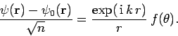
It follows that neither the incident wavefunction,
 |
(1283) |
nor the large- form of the total wavefunction,
![\begin{displaymath}
\psi({\bf r}) = \sqrt{n}
\left[ \exp( {\rm i} k r\cos\theta) + \frac{\exp( {\rm i} k r) f(\theta)}
{r} \right],
\end{displaymath}](img2906.png) |
(1284) |
depend on the azimuthal angle .
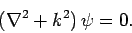
Outside the range of the scattering potential, both
 and
and
 satisfy the free space Schrödinger equation
 |
(1285) |
What is the most general solution to this equation in spherical polar
coordinates which does not depend on the azimuthal angle ?
Separation of variables yields
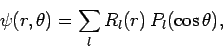 |
(1286) |
since the Legendre functions
 form a complete
set in -space. The Legendre functions are related to the
spherical harmonics, introduced in Cha. 8, via
form a complete
set in -space. The Legendre functions are related to the
spherical harmonics, introduced in Cha. 8, via
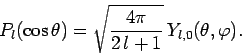 |
(1287) |
Equations (1285) and (1286) can be combined to give
![\begin{displaymath}
r^2 \frac{d^2 R_l}{dr^2} + 2 r \frac{dR_l}{dr} + [k^2 r^2 -
l (l+1)]R_l = 0.
\end{displaymath}](img2911.png) |
(1288) |
The two independent solutions to this equation are the
spherical Bessel functions,  and
and
 , introduced in Sect. 9.3.
Recall that
, introduced in Sect. 9.3.
Recall that
Note that the  are well-behaved in the limit
 , whereas the
  become singular.
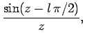
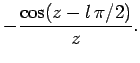
The asymptotic behaviour of these functions in the limit
become singular.
The asymptotic behaviour of these functions in the limit
 is
is
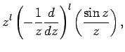
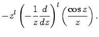
We can write
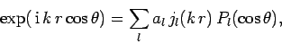 |
(1293) |
where the  are constants. Note there are no functions in
this expression, because they are not well-behaved as
are constants. Note there are no functions in
this expression, because they are not well-behaved as
 .
The Legendre functions are orthonormal,
.
The Legendre functions are orthonormal,
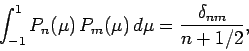 |
(1294) |
so we can invert the above expansion to give
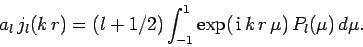 |
(1295) |
It is well-known that
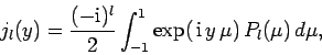 |
(1296) |
where
 [see M. Abramowitz and I.A. Stegun, Handbook of mathematical functions, (Dover, New York NY, 1965),
Eq. 10.1.14]. Thus,
[see M. Abramowitz and I.A. Stegun, Handbook of mathematical functions, (Dover, New York NY, 1965),
Eq. 10.1.14]. Thus,
 |
(1297) |
giving
 |
(1298) |
The above expression tells us how to decompose
the incident plane-wave into
a series of spherical waves. These waves are usually termed ``partial waves''.
The most general expression for the total wavefunction outside the
scattering region is
![\begin{displaymath}
\psi({\bf r}) = \sqrt{n}\sum_l\left[
A_l j_l(k r) + B_l y_l(k r)\right] P_l(\cos\theta),
\end{displaymath}](img2923.png) |
(1299) |
where the  and
and  are constants.
Note that the functions are allowed to appear
in this expansion, because
its region of validity does not include the origin. In the large-
limit, the total wavefunction reduces to
are constants.
Note that the functions are allowed to appear
in this expansion, because
its region of validity does not include the origin. In the large-
limit, the total wavefunction reduces to
![\begin{displaymath}
\psi ({\bf r} ) \simeq \sqrt{n} \sum_l\left[A_l
\frac{\sin...
..._l \frac{\cos(k r -l \pi/2)}{k r}
\right] P_l(\cos\theta),
\end{displaymath}](img2926.png) |
(1300) |
where use has been made of Eqs. (1291) and (1292). The above expression can also
be written
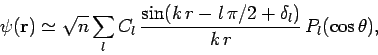 |
(1301) |
where the sine and cosine functions have been combined to give a
sine function which is phase-shifted by  . Note that
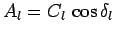 and
and
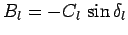 .
.
Equation (1301) yields
![\begin{displaymath}
\psi({\bf r}) \simeq \sqrt{n} \sum_l C_l\left[
\frac{{\rm e}...
...\pi/2+ \delta_l)} }{2 {\rm i} k r} \right] P_l(\cos\theta),
\end{displaymath}](img2931.png) |
(1302) |
which contains both incoming and outgoing spherical waves. What is the
source of the incoming waves? Obviously, they must be part of
the large- asymptotic expansion of the incident wavefunction. In fact,
it is easily seen from Eqs. (1291) and (1298)
that
![\begin{displaymath}
\psi_0({\bf r}) \simeq \sqrt{n} \sum_l {\rm i}^{ l}
(2l+1...
... (k r - l \pi/2)}}{2 {\rm i} k r} \right]P_l(\cos\theta)
\end{displaymath}](img2932.png) |
(1303) |
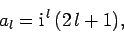
in the large- limit. Now, Eqs. (1283) and (1284) give
 |
(1304) |
Note that the right-hand side consists of an outgoing spherical
wave only. This implies that the coefficients of the incoming spherical waves
in the large- expansions of and
must be the same. It follows from Eqs. (1302) and (1303) that
![\begin{displaymath}
C_l = (2 l+1) \exp[ {\rm i} (\delta_l + l \pi/2)].
\end{displaymath}](img2934.png) |
(1305) |
Thus, Eqs. (1302)-(1304) yield
 |
(1306) |
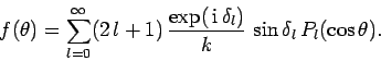
Clearly, determining the scattering amplitude
 via a decomposition into
partial waves (i.e., spherical waves) is equivalent to determining
the phase-shifts .
via a decomposition into
partial waves (i.e., spherical waves) is equivalent to determining
the phase-shifts .
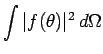
Now, the differential scattering cross-section
 is simply
the modulus squared of the scattering amplitude [see Eq. (1266)]. The
total cross-section is thus given by
is simply
the modulus squared of the scattering amplitude [see Eq. (1266)]. The
total cross-section is thus given by
where
 . It follows that
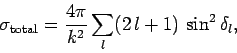 |
(1308) |
where use has been made of Eq. (1294).
Next: Determination of Phase-Shifts
Up: Scattering Theory
Previous: Born Approximation
Richard Fitzpatrick
2010-07-20
![$\displaystyle \frac{1}{k^2} \oint d\phi \int_{-1}^{1} d\mu
\sum_l \sum_{l'} (2 l+1) (2 l'+1)
\exp[ {\rm i} (\delta_l-\delta_{l'})]$](img2938.png)