Determination of Phase-Shifts

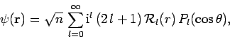
Let us now consider how the phase-shifts $\delta_l$ in Eq. (1306) can be evaluated. Consider a spherically symmetric potential $V(r)$ which vanishes for $r>a$, where $a$ is termed the range of the potential. In the region $r>a$, the wavefunction $\psi({\bf r})$ satisfies the free-space Schrödinger equation (1285). The most general solution which is consistent with no incoming spherical-waves is

$$\psi({\bf r}) = \sqrt{n} \sum_{l=0}^\infty {\rm i}^l (2 l+1) {\cal R}_l(r) P_l(\cos\theta),$$ (1309)

where

$${\cal R}_l(r) = \exp( {\rm i} \delta_l) \left[\cos\delta_l j_l(k r) -\sin\delta_l y_l(k r)\right].$$ (1310)

Note that $y_l(k r)$ functions are allowed to appear in the above expression, because its region of validity does not include the origin (where $V\neq 0$). The logarithmic derivative of the $l$th radial wavefunction, ${\cal R}_l(r)$, just outside the range of the potential is given by

$$\beta_{l+} = k a \left[\frac{ \cos\delta_l j_l'(k a) - \s... ...}{\cos\delta_l j_l(k a) - \sin\delta_l y_l(k a)}\right],$$ (1311)

where $j_l'(x)$ denotes $dj_l(x)/dx$, etc. The above equation can be inverted to give

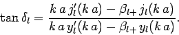$$\tan \delta_l = \frac{ k a j_l'(k a) - \beta_{l+} j_l(k a)} {k a y_l'(k a) - \beta_{l+} y_l(k a)}.$$ (1312)

Thus, the problem of determining the phase-shift $\delta_l$ is equivalent to that of obtaining $\beta_{l+}$.

The most general solution to Schrödinger's equation inside the range of the potential ($r<a$) which does not depend on the azimuthal angle $\phi$ is

$$\psi({\bf r}) = \sqrt{n} \sum_{l=0}^\infty {\rm i}^{ l} (2 l+1) {\cal R}_l(r) P_l(\cos\theta),$$ (1313)

where

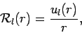$${\cal R}_l (r) = \frac{u_l(r)}{r},$$ (1314)

and

$$\frac{d^2 u_l}{d r^2} +\left[k^2 -\frac{l (l+1)}{r^2} -\frac{2 m}{\hbar^2} V\right] u_l = 0.$$ (1315)

The boundary condition

$$u_l(0) = 0$$ (1316)

ensures that the radial wavefunction is well-behaved at the origin. We can launch a well-behaved solution of the above equation from $r=0$, integrate out to $r=a$, and form the logarithmic derivative

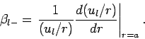$$\beta_{l-} = \left.\frac{1}{(u_l/r)} \frac{d(u_l/r)}{dr}\right\vert _{r=a}.$$ (1317)

Since $\psi({\bf r})$ and its first derivatives are necessarily continuous for physically acceptible wavefunctions, it follows that

$$\beta_{l+} = \beta_{l-}.$$ (1318)

The phase-shift $\delta_l$ is then obtainable from Eq. (1312).