Next: Spin Precession
Up: Spin Angular Momentum
Previous: Eigenstates of and
Pauli Representation
Let us denote the two independent spin eigenstates of an electron as
 |
(734) |
It thus follows, from Eqs. (717) and (718), that
Note that  corresponds to an electron whose spin angular momentum vector has a positive component along the
  -axis. Loosely speaking,
we could say that the spin vector points in the
-axis. Loosely speaking,
we could say that the spin vector points in the  -direction (or its spin is
``up''). Likewise,
-direction (or its spin is
``up''). Likewise,
 corresponds to an electron whose spin points in the
  -direction
(or whose spin is ``down'').
These two eigenstates satisfy the orthonormality requirements
-direction
(or whose spin is ``down'').
These two eigenstates satisfy the orthonormality requirements
 |
(737) |
and
 |
(738) |
A general spin state can be represented as a linear combination of
and : i.e.,
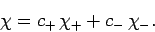 |
(739) |
It is thus evident that electron spin space is two-dimensional.
Up to now, we have discussed spin space in rather abstract terms. In the
following, we shall describe a particular representation of electron
spin space due to Pauli. This so-called Pauli representation allows us
to visualize spin space, and also facilitates calculations involving spin.
Let us attempt to represent a general spin state as a complex column vector in some two-dimensional space: i.e.,
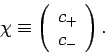 |
(740) |
The corresponding dual vector is represented as a row vector: i.e.,
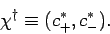 |
(741) |
Furthermore, the product
 is obtained according to the
ordinary rules of matrix multiplication: i.e.,
is obtained according to the
ordinary rules of matrix multiplication: i.e.,
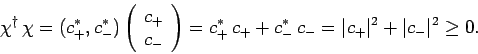 |
(742) |
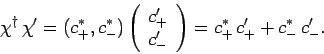
Likewise, the product
 of two different spin states
is also obtained from the rules of matrix multiplication: i.e.,
of two different spin states
is also obtained from the rules of matrix multiplication: i.e.,
 |
(743) |
Note that this particular representation of spin space is in complete accordance with the discussion in Sect. 10.3. For obvious reasons,
a vector used to represent a spin state is generally known as
spinor.
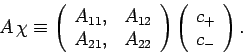
A general spin operator  is represented as a
  matrix
which operates on a spinor: i.e.,
matrix
which operates on a spinor: i.e.,
 |
(744) |
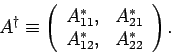
As is easily demonstrated, the Hermitian conjugate of is represented by
the transposed complex conjugate of the matrix used to represent : i.e.,
 |
(745) |
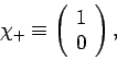
Let us represent the spin eigenstates and as
 |
(746) |
and
 |
(747) |
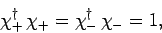
respectively. Note that these forms automatically
satisfy the orthonormality constraints (737) and (738).
It is convenient to write the spin operators  (where
  corresponds to
 ) as
) as
 |
(748) |
Here, the  are dimensionless matrices. According
to Eqs. (702)-(704), the satisfy the commutation
relations
are dimensionless matrices. According
to Eqs. (702)-(704), the satisfy the commutation
relations
Furthermore, Eq. (735) yields
 |
(752) |
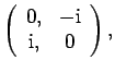
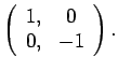
It is easily demonstrated, from the above expressions, that the are represented by the
following matrices:
Incidentally, these matrices are generally known as the Pauli matrices.
Finally, a general spinor takes the form
 |
(756) |
If the spinor is properly normalized then
 |
(757) |
In this case, we can interpret  as the probability that
an observation of
as the probability that
an observation of  will yield the result
  , and
, and
 as the probability that an observation of
will yield the result
as the probability that an observation of
will yield the result  .
.
Next: Spin Precession
Up: Spin Angular Momentum
Previous: Eigenstates of and
Richard Fitzpatrick
2010-07-20