


Next: Exercises
Up: Spin Angular Momentum
Previous: Pauli Representation
Spin Precession
According to classical physics, a small current loop possesses a magnetic moment of magnitude  , where
 is the current circulating around the loop, and
  the area of the loop.
The direction of the magnetic moment is conventionally taken to be
normal to the plane of the loop, in the sense given by a standard
right-hand circulation rule. Consider a small current loop consisting of an electron in uniform circular motion. It is
easily demonstrated that the electron's orbital angular momentum
the area of the loop.
The direction of the magnetic moment is conventionally taken to be
normal to the plane of the loop, in the sense given by a standard
right-hand circulation rule. Consider a small current loop consisting of an electron in uniform circular motion. It is
easily demonstrated that the electron's orbital angular momentum  is related to the magnetic moment
 of the loop via
 |
(758) |
where  is the magnitude of the electron charge, and
  the electron mass.
The above expression suggests that there may be a similar relationship between
magnetic moment and spin angular momentum. We can write
 |
(759) |
where  is called the gyromagnetic ratio. Classically, we would
expect
is called the gyromagnetic ratio. Classically, we would
expect  . In fact,
 |
(760) |
where
 is the so-called
fine-structure constant. The fact that the gyromagnetic ratio is
(almost) twice that expected from classical physics is only explicable using relativistic
quantum mechanics. Furthermore, the small corrections to the relativistic result
is the so-called
fine-structure constant. The fact that the gyromagnetic ratio is
(almost) twice that expected from classical physics is only explicable using relativistic
quantum mechanics. Furthermore, the small corrections to the relativistic result  come from quantum field theory.
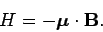
The energy of a classical magnetic moment
in a uniform magnetic field  is
is
 |
(761) |
Assuming that the above expression also holds good in quantum mechanics,
the Hamiltonian of an electron in a  -directed magnetic field of magnitude
 takes the form
 |
(762) |
where
 |
(763) |
Here, for the sake of simplicity, we are neglecting the electron's translational degrees of freedom.
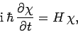
Schrödinger's equation can be written
[see Eq. (199)]
 |
(764) |
where the spin state of the electron is characterized by the spinor  .
Adopting the Pauli representation, we obtain
.
Adopting the Pauli representation, we obtain
 |
(765) |
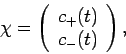
where
 . Here,
  is the probability of observing the
spin-up state, and
is the probability of observing the
spin-up state, and  the probability of observing the spin-down
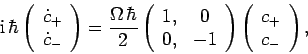
state. It follows from Eqs. (748), (755), (762),
(764), and (765) that
the probability of observing the spin-down
state. It follows from Eqs. (748), (755), (762),
(764), and (765) that
 |
(766) |
where
 .
Hence,
.
Hence,
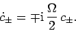 |
(767) |
Let
The significance of the angle  will become apparent presently.
Solving Eq. (767), subject to the initial conditions
(768) and (769), we obtain
will become apparent presently.
Solving Eq. (767), subject to the initial conditions
(768) and (769), we obtain
We can most easily visualize the effect of the time dependence in the above
expressions for  by calculating the expectation
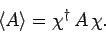
values of the three Cartesian components of the electron's spin angular momentum. By analogy
with Eq. (192), the expectation value of a general spin operator
is simply
by calculating the expectation
values of the three Cartesian components of the electron's spin angular momentum. By analogy
with Eq. (192), the expectation value of a general spin operator
is simply
 |
(772) |
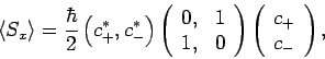
Hence, the expectation value of  is
is
 |
(773) |
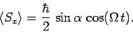
which reduces to
 |
(774) |
with the help of Eqs. (770) and (771). Likewise,
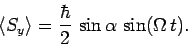
the expectation value of  is
is
 |
(775) |
which reduces to
 |
(776) |
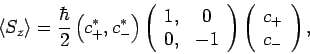
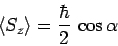
Finally, the expectation value of  is
is
 |
(777) |
According to Eqs. (774), (776), and (777),
the expectation value of the spin angular momentum vector subtends
a constant angle with the -axis, and precesses about
this axis at the frequency
 |
(778) |
This behaviour is actually equivalent to that predicted by classical physics.
Note, however, that a measurement of , , or will always
yield either  or
or  . It is the relative probabilities
of obtaining these two results which varies as the expectation value
of a given component of the spin varies.
. It is the relative probabilities
of obtaining these two results which varies as the expectation value
of a given component of the spin varies.
Subsections
Next: Exercises
Up: Spin Angular Momentum
Previous: Pauli Representation
Richard Fitzpatrick
2010-07-20