


Next: Zeeman Effect
Up: Time-Independent Perturbation Theory
Previous: Linear Stark Effect
Fine Structure of Hydrogen
According to special relativity, the kinetic energy (i.e., the difference
between the total energy and the rest mass energy) of a particle
of rest mass  and momentum
  is
is
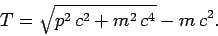 |
(966) |
In the non-relativistic limit  , we can expand the square-root
in the above expression to give
, we can expand the square-root
in the above expression to give
![\begin{displaymath}
T = \frac{p^2}{2 m}\left[1- \frac{1}{4}\left(\frac{p}{m c}\right)^2+
{\cal O}\left(\frac{p}{m c}\right)^4\right].
\end{displaymath}](img2290.png) |
(967) |
Hence,
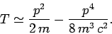 |
(968) |
Of course, we recognize the first term on the right-hand side of this equation
as the standard non-relativistic expression for the kinetic energy.
The second term is the lowest-order relativistic correction to this
energy. Let us consider the effect of this type of correction on the energy
levels of a hydrogen atom. So, the unperturbed Hamiltonian is
given by Eq. (911), and the perturbing Hamiltonian
takes the form
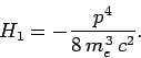 |
(969) |
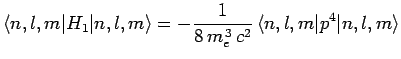
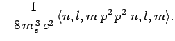
Now, according to standard first-order perturbation theory (see Sect. 12.4), the lowest-order relativistic correction to the energy of a hydrogen atom state characterized
by the standard quantum numbers  ,
,  , and is given by
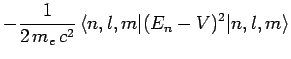
However, Schrödinger's equation for a unperturbed hydrogen atom
can be written
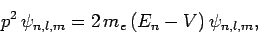 |
(971) |
where
 .
Since
.
Since  is an Hermitian operator, it follows that
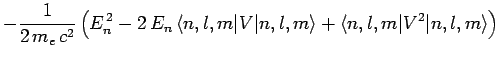
It follows from Eqs. (695) and (696) that
Finally, making use of Eqs. (676), (678), and (679), the above expression reduces to
 |
(974) |
where
 |
(975) |
is the dimensionless fine structure constant.
Note that the above derivation implicitly assumes that  is an Hermitian
operator. It turns out that this is not the case for
is an Hermitian
operator. It turns out that this is not the case for  states. However,
somewhat fortuitously,
our calculation still gives the correct answer when . Note, also,
that we are able to use non-degenerate perturbation theory in the
above calculation, using the
states. However,
somewhat fortuitously,
our calculation still gives the correct answer when . Note, also,
that we are able to use non-degenerate perturbation theory in the
above calculation, using the  eigenstates, because the perturbing Hamiltonian commutes
with both
eigenstates, because the perturbing Hamiltonian commutes
with both  and
and  . It follows that there is no
coupling between states with different and quantum numbers.
Hence, all coupled states have different quantum numbers, and
therefore have different energies.
. It follows that there is no
coupling between states with different and quantum numbers.
Hence, all coupled states have different quantum numbers, and
therefore have different energies.
Now, an electron in a hydrogen atom experiences an electric field
 |
(976) |
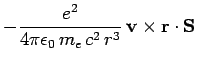
due to the charge on the nucleus. However, according to
electromagnetic theory, a non-relativistic particle moving in a
electric field  with velocity
  also experiences an effective
magnetic field
also experiences an effective
magnetic field
 |
(977) |
Recall, that an electron possesses a magnetic moment [see Eqs. (759)
and (760)]
 |
(978) |
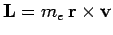
due to its spin angular momentum,  . We, therefore, expect
an additional contribution to the Hamiltonian of a hydrogen atom of the form [see Eq. (761)]
. We, therefore, expect
an additional contribution to the Hamiltonian of a hydrogen atom of the form [see Eq. (761)]
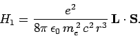
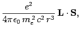
where
 is the electron's orbital angular momentum. This effect is known as spin-orbit coupling. It turns
out that the above expression is too large, by a factor 2, due to an
obscure relativistic effect known as Thomas precession. Hence, the true
spin-orbit correction to the Hamiltonian is
is the electron's orbital angular momentum. This effect is known as spin-orbit coupling. It turns
out that the above expression is too large, by a factor 2, due to an
obscure relativistic effect known as Thomas precession. Hence, the true
spin-orbit correction to the Hamiltonian is
 |
(980) |
Let us now apply perturbation theory to the hydrogen atom, using the
above expression as the perturbing Hamiltonian.
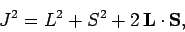
Now
 |
(981) |
is the total angular momentum of the system. Hence,
 |
(982) |
giving
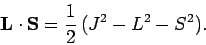 |
(983) |
Recall, from Sect. 11.2, that whilst  commutes with both
and
commutes with both
and  , it does not commute with either or
  . It follows
that the perturbing Hamiltonian (980) also commutes with both and , but does not commute with either or .
Hence, the simultaneous eigenstates of the unperturbed Hamiltonian (911)
and the perturbing Hamiltonian (980) are the same as the simultaneous
eigenstates of , , and discussed in Sect. 11.3.
It is important to know this since, according to Sect. 12.6, we
can only safely apply perturbation theory to the simultaneous
eigenstates of the unperturbed and perturbing Hamiltonians.
. It follows
that the perturbing Hamiltonian (980) also commutes with both and , but does not commute with either or .
Hence, the simultaneous eigenstates of the unperturbed Hamiltonian (911)
and the perturbing Hamiltonian (980) are the same as the simultaneous
eigenstates of , , and discussed in Sect. 11.3.
It is important to know this since, according to Sect. 12.6, we
can only safely apply perturbation theory to the simultaneous
eigenstates of the unperturbed and perturbing Hamiltonians.
Adopting the notation introduced in Sect. 11.3, let
 be a simultaneous eigenstate of , ,
, and
be a simultaneous eigenstate of , ,
, and  corresponding to the eigenvalues
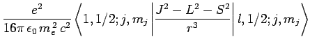
According to standard first-order perturbation theory, the energy-shift induced in such a state
by spin-orbit coupling is given by
Here, we have made use of the fact that  for an electron. It follows
from Eq. (697) that
for an electron. It follows
from Eq. (697) that
![\begin{displaymath}
\Delta E_{l,1/2;j,m_j}= \frac{e^2 \hbar^2}{16\pi \epsilon_...
...t[\frac{j (j+1)-l (l+1)-3/4}{l (l+1/2) (l+1) n^3}\right],
\end{displaymath}](img2323.png) |
(989) |
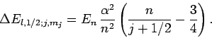
where is the radial quantum number. Finally, making use of Eqs. (676), (678), and (679), the above expression reduces to
![\begin{displaymath}
\Delta E_{l,1/2;j,m_j}= E_n \frac{\alpha^2}{n^2}\left[
\fra...
...\{3/4+l (l+1)-j (j+1)\right\}}{2 l (l+1/2) (l+1)}\right],
\end{displaymath}](img2324.png) |
(990) |
where  is the fine structure constant. A comparison of this
expression with Eq. (974) reveals that the energy-shift
due to spin-orbit coupling is of the same order of magnitude as that due
to the lowest-order relativistic correction to the Hamiltonian. We can
add these two corrections together (making use of the fact that
is the fine structure constant. A comparison of this
expression with Eq. (974) reveals that the energy-shift
due to spin-orbit coupling is of the same order of magnitude as that due
to the lowest-order relativistic correction to the Hamiltonian. We can
add these two corrections together (making use of the fact that
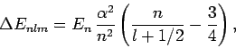
 for a hydrogen atom--see Sect. 11.3) to obtain
a net energy-shift of
for a hydrogen atom--see Sect. 11.3) to obtain
a net energy-shift of
 |
(991) |
This modification of the energy levels of a hydrogen atom due to a combination
of relativity and spin-orbit coupling is
known as fine structure.
Now, it is conventional to refer to the energy eigenstates of a hydrogen
atom which are also simultaneous eigenstates of as  states,
where is the radial quantum number,
states,
where is the radial quantum number,
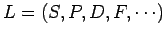 as
as
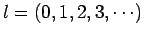 , and
, and  is the total angular momentum quantum number.
Let us examine the effect of the fine structure energy-shift (991)
on these eigenstates for
is the total angular momentum quantum number.
Let us examine the effect of the fine structure energy-shift (991)
on these eigenstates for  and 3.
For  , in the absence of fine structure, there are two degenerate
  states.
According to Eq. (991), the fine structure induced energy-shifts of
these two states are the same. Hence, fine structure does not
break the degeneracy of the two states of hydrogen.
states.
According to Eq. (991), the fine structure induced energy-shifts of
these two states are the same. Hence, fine structure does not
break the degeneracy of the two states of hydrogen.
For  , in the absence of fine structure, there are two
  states, two
  states, and four
  states, all
of which are degenerate.
According to Eq. (991), the fine structure induced energy-shifts of
the and states are the same as one another, but are different
from the induced
energy-shift of the states.
Hence, fine structure does not break the
degeneracy of the and states of hydrogen, but
does break the degeneracy of these states relative to the
states.
states, all
of which are degenerate.
According to Eq. (991), the fine structure induced energy-shifts of
the and states are the same as one another, but are different
from the induced
energy-shift of the states.
Hence, fine structure does not break the
degeneracy of the and states of hydrogen, but
does break the degeneracy of these states relative to the
states.
For  , in the absence of fine structure, there are two
  states, two
  states, four
  states, four
  states, and six
  states, all of
which are degenerate. According to Eq. (991), fine structure
breaks these states into three groups: the and states,
the and states, and the states.
states, all of
which are degenerate. According to Eq. (991), fine structure
breaks these states into three groups: the and states,
the and states, and the states.
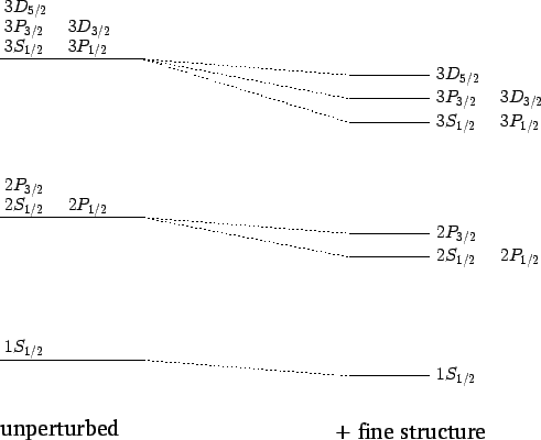
The effect of the fine structure energy-shift on the , 2, and 3 energy
states of a hydrogen atom is illustrated in Fig. 23.
Figure 23:
Effect of the fine structure energy-shift on the
and 3 states of a hydrogen atom. Not to scale.
 |
Note, finally, that although expression (990) does not
have a well-defined value for , when added to expression (974) it, somewhat fortuitously, gives rise to an expression
(991) which is both well-defined and correct when .
Next: Zeeman Effect
Up: Time-Independent Perturbation Theory
Previous: Linear Stark Effect
Richard Fitzpatrick
2010-07-20
![$\displaystyle -\frac{1}{2 m_e c^2}\left[
E_n^{ 2} + 2 E_n\left(\frac{e^2}{4...
...e^2}{4\pi\epsilon_0}\right)^2\left\langle\frac{1}{r^{ 2}}\right\rangle\right].$](img2300.png)
![$\displaystyle -\frac{1}{2 m_e c^2}\left[
E_n^{ 2} + 2 E_n\left(\frac{e^2}{4...
...ft(\frac{e^2}{4\pi\epsilon_0}\right)^2\frac{1}{(l+1/2) n^3 a_0^{ 2}}\right].$](img2301.png)
![$\displaystyle \frac{e^2 \hbar^2}{16\pi \epsilon_0 m_e^{ 2} c^2} \left[j (j+1)-l (l+1)-3/4\right] \left\langle\frac{1}{r^3}\right\rangle.$](img2322.png)