Spin Greater Than One-Half Systems

In the absence of spin, the Hamiltonian can be written as some function of the position and momentum operators. Using the Schrödinger representation, in which ${\bf p} \rightarrow -{\rm i}\,\hbar\,\nabla$ , the energy eigenvalue problem,

$$H\,\vert E\rangle = E\,\vert E\rangle,$$ (520)

can be transformed into a partial differential equation for the wavefunction $\psi({\bf x}') \equiv \langle {\bf x'}\vert E\rangle$ . This function specifies the probability density for observing the particle at a given position, ${\bf x}'$ . In general, we find

$$H\,\psi = E\,\psi,$$ (521)

where $H$ is now a partial differential operator. The boundary conditions (for a bound state) are obtained from the normalization constraint

$$\int d^3x'\, \vert\psi\vert^{\,2}= 1.$$ (522)

This is all very familiar. However, we now know how to generalize this scheme to deal with a spin one-half particle. Instead of representing the state of the particle by a single wavefunction, we use two wavefunctions. The first, $\psi_+({\bf x'})$ , specifies the probability density of observing the particle at position ${\bf x}'$ with spin angular momentum $+\hbar/2$ in the $z$ -direction. The second, $\psi_-({\bf x'})$ , specifies the probability density of observing the particle at position ${\bf x}'$ with spin angular momentum $-\hbar/2$ in the $z$ -direction. In the Pauli scheme, these wavefunctions are combined into a spinor, $\chi$ , which is simply the column vector of $\psi_+$ and $\psi_-$ . In general, the Hamiltonian is a function of the position, momentum, and spin operators. Adopting the Schrödinger representation, and the Pauli scheme, the energy eigenvalue problem reduces to

$$H \,\chi = E \,\chi,$$ (523)

where $\chi$ is a spinor (i.e., a $2\times 1$ matrix of wavefunctions) and $H$ is a $2\times 2$ matrix partial differential operator [see Equation (507)]. The above spinor equation can always be written out explicitly as two coupled partial differential equations for $\psi_+$ and $\psi_-$ .

Suppose that the Hamiltonian has no dependence on the spin operators. In this case, the Hamiltonian is represented as diagonal $2\times 2$ matrix partial differential operator in the Schrödinger/Pauli scheme [see Equation (506)]. In other words, the partial differential equation for $\psi_+$ decouples from that for $\psi_-$ . In fact, both equations have the same form, so there is only really one differential equation. In this situation, the most general solution to Equation (523) can be written

$$\chi = \psi({\bf x}') \left(\!\begin{array}{c} c_+\\ c_-\end{array}\!\right).$$ (524)

Here, $\psi({\bf x}')$ is determined by the solution of the differential equation, and the $c_\pm$ are arbitrary complex numbers. The physical significance of the above expression is clear. The Hamiltonian determines the relative probabilities of finding the particle at various different positions, but the direction of its spin angular momentum remains undetermined.

Suppose that the Hamiltonian depends only on the spin operators. In this case, the Hamiltonian is represented as a $2\times 2$ matrix of complex numbers in the Schrödinger/Pauli scheme [see Equation (489)], and the spinor eigenvalue equation (523) reduces to a straightforward matrix eigenvalue problem. The most general solution can again be written

$$\chi = \psi({\bf x}') \left(\!\begin{array}{c} c_+\\ c_-\end{array}\!\right).$$ (525)

Here, the ratio $c_+/c_-$ is determined by the matrix eigenvalue problem, and the wavefunction $\psi({\bf x}')$ is arbitrary. Clearly, the Hamiltonian determines the direction of the particle's spin angular momentum, but leaves its position undetermined.

In general, of course, the Hamiltonian is a function of both position and spin operators. In this case, it is not possible to decompose the spinor as in Equations (524) and (525). In other words, a general Hamiltonian causes the direction of the particle's spin angular momentum to vary with position in some specified manner. This can only be represented as a spinor involving different wavefunctions, $\psi_+$ and $\psi_-$ .

But, what happens if we have a spin one or a spin three-halves particle? It turns out that we can generalize the Pauli two-component scheme in a fairly straightforward manner. Consider a spin-$s$ particle: i.e., a particle for which the eigenvalue of $S^2$ is $s\,(s+1)\,\hbar^2$ . Here, $s$ is either an integer, or a half-integer. The eigenvalues of $S_z$ are written $s_z\,\hbar$ , where $s_z$ is allowed to take the values $s, s-1, \cdots, -s+1, -s$ . In fact, there are $2\,s+1$ distinct allowed values of $s_z$ . Not surprisingly, we can represent the state of the particle by $2\,s+1$ different wavefunctions, denoted $\psi_{s_z} ({\bf x}')$ . Here, $\psi_{s_z} ({\bf x}')$ specifies the probability density for observing the particle at position ${\bf x'}$ with spin angular momentum $s_z\,\hbar$ in the $z$ -direction. More exactly,

$$\psi_{s_z}({\bf x}') = \langle {\bf x'}\vert\langle s, s_z\vert \vert A\rangle\rangle,$$ (526)

where $\vert\vert A\rangle\rangle$ denotes a state ket in the product space of the position and spin operators. The state of the particle can be represented more succinctly by a spinor, $\chi$ , which is simply the $2\,s+1$ component column vector of the $\psi_{s_z} ({\bf x}')$ . Thus, a spin one-half particle is represented by a two-component spinor, a spin one particle by a three-component spinor, a spin three-halves particle by a four-component spinor, and so on.

In this extended Schrödinger/Pauli scheme, position space operators take the form of diagonal $(2\,s+1) \times (2\,s+1)$ matrix differential operators. Thus, we can represent the momentum operators as [see Equation (506)]

$$p_k \rightarrow -{\rm i}\,\hbar \,\frac{\partial}{\partial x_k'}\, {\bf 1},$$ (527)

where ${\bf 1}$ is the $(2\,s+1) \times (2\,s+1)$ unit matrix. We represent the spin operators as

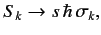$$S_k \rightarrow s\,\hbar \,\sigma_k,$$ (528)

where the $(2\,s+1) \times (2\,s+1)$ extended Pauli matrix $\sigma_k$ has elements

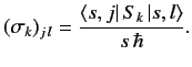$$(\sigma_k)_{j\,l} = \frac{ \langle s, j\vert\,S_k\, \vert s, l\rangle}{s\,\hbar}.$$ (529)

Here, $j, l$ are integers, or half-integers, lying in the range $-s$ to $+s$ . But, how can we evaluate the brackets $\langle s, j\vert\,S_k \,\vert s, l\rangle$ and, thereby, construct the extended Pauli matrices? In fact, it is trivial to construct the $\sigma_z$ matrix. By definition,

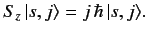$$S_z\, \vert s, j\rangle = j\,\hbar\, \vert s, j\rangle.$$ (530)

Hence,

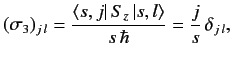$$(\sigma_3)_{j\,l} = \frac{\langle s, j\vert\,S_z\, \vert s, l\rangle}{s\,\hbar} = \frac{j}{s}\, \delta_{j\,l},$$ (531)

where use has been made of the orthonormality property of the $\vert s, j\rangle$ . Thus, $\sigma_z$ is the suitably normalized diagonal matrix of the eigenvalues of $S_z$ . The matrix elements of $\sigma_x$ and $\sigma_y$ are most easily obtained by considering the shift operators,

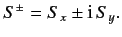$$S^\pm = S_x \pm {\rm i}\, S_y.$$ (532)

We know, from Equations (344)-(345), that

$$S^+\, \vert s, j\rangle = [s\,(s+1) - j \,(j+1)]^{1/2} \,\hbar\, \vert s, j+1\rangle,$$ (533)

$$S^- \,\vert s, j\rangle = [s\,(s+1) - j \,(j-1)]^{1/2}\, \hbar \,\vert s, j-1\rangle.$$ (534)

It follows from Equations (529), and (532)-(534), that

$$(\sigma_1)_{j\,l} = \frac{[s\,(s+1) - j\,(j-1)]^{1/2} }{2\,s}\,\delta_{j\,\, l+1}+ \frac{[s\,(s+1) - j\,(j+1)]^{1/2} }{2\,s}\,\delta_{j\,\, l-1},$$ (535)

$$(\sigma_2)_{j\,l} = \frac{[ s\,(s+1) - j\,(j-1)]^{1/2} }{2\,{\rm i}\,s}\,\delta_{j\,\, l+1}- \frac{[s\,(s+1) - j\,(j+1)]^{1/2} }{2\,{\rm i}\,s}\,\delta_{j\,\, l-1}.$$ (536)

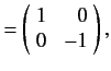
According to Equations (531) and (535)-(536), the Pauli matrices for a spin one-half ($s=1/2$ ) particle are

$$\sigma_1 = \left(\!\begin{array}{rr} 0 &1\\ 1&0\end{array}\!\right),$$ (537)

$$\sigma_2 = \left(\!\begin{array}{rr} 0 &-{\rm i}\\ {\rm i}&0\end{array}\!\right),$$ (538)

$$\sigma_3 = \left(\!\begin{array}{rr} 1 &0\\ 0&-1\end{array}\!\right),$$ (539)

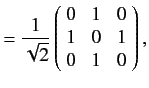
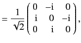
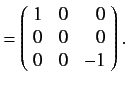
as we have seen previously. For a spin one ($s=1$ ) particle, we find that

$$\sigma_1 =\frac{1}{\sqrt{2}}\left(\! \begin{array}{rrr} 0 &1&0\\ 1&0&1\\ 0&1&0\end{array}\!\right),$$ (540)

$$\sigma_2 = \frac{1}{\sqrt{2}} \left(\!\begin{array}{rrr} 0 &-{\rm i}&0\\ {\rm i}&0&{-\rm i}\\ 0&{\rm i}& 0\end{array}\!\right),$$ (541)

$$\sigma_3 = \left(\!\begin{array}{rrr} 1 &0&0\\ 0&0&0\\ 0&0&-1\end{array}\!\right).$$ (542)

In fact, we can now construct the Pauli matrices for a spin anything particle. This means that we can convert the general energy eigenvalue problem for a spin-$s$ particle, where the Hamiltonian is some function of position and spin operators, into $2\,s+1$ coupled partial differential equations involving the $2\,s+1$ wavefunctions $\psi_{s_z}({\bf x'})$ . Unfortunately, such a system of equations is generally too complicated to solve exactly.