Two-State System

Consider a system in which the time-independent Hamiltonian possesses two eigenstates, denoted

$$H_0 \,\vert 1\rangle = E_1 \,\vert 1\rangle,$$ (8.13)

$$H_0 \,\vert 2\rangle = E_2 \,\vert 2\rangle,$$ (8.14)

where $E_2>E_1$ . Suppose, for the sake of simplicity, that the diagonal matrix elements of the interaction Hamiltonian, $H_1$ , are zero: that is,

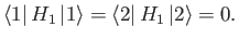$$\langle 1\vert\,H_1\,\vert 1\rangle = \langle 2\vert\,H_1\,\vert 2\rangle = 0.$$ (8.15)

The off-diagonal matrix elements are assumed to oscillate sinusoidally at some angular frequency $\omega$ :

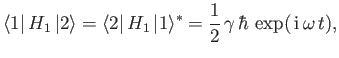$$\langle 1\vert\,H_1\,\vert 2\rangle = \langle 2\vert\,H_1\,\vert 1\rangle^\ast = \frac{1}{2}\,\gamma\,\hbar\, \exp(\,{\rm i}\, \omega\,t),$$ (8.16)

where $\gamma$ and $\omega$ are real. Note that it is only the off-diagonal matrix elements that give rise to the effect in which we are primarily interested--namely, transitions between states 1 and 2. (See Exercise 1.)

For a two-state system, Equation (8.11) reduces to

$${\rm i} \, \frac{d c_1}{dt} = \frac{\gamma}{2}\,\exp[+{\rm i}\, (\omega-\omega_{21})\,t\,]\,c_2,$$ (8.17)

$${\rm i}\, \frac{d c_2}{dt} =\frac{\gamma}{2}\, \exp[-{\rm i}\, (\omega-\omega_{21})\,t\,]\,c_1,$$ (8.18)

where $\omega_{21} = (E_2 - E_1)/\hbar$ , and it is assumed that $t_0=0$ . Equations (8.18) and (8.19) can be combined to give a second-order differential equation for the time variation of the amplitude $c_2$ :

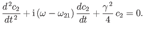$$\frac{d^{\,2} c_2}{dt^{\,2}} + {\rm i}\,(\omega-\omega_{21})\,\frac{d c_2}{dt} + \frac{\gamma^{\,2}}{4} \,c_2 = 0.$$ (8.19)

Once we have solved for $c_2$ , we can use Equation (8.19) to obtain the amplitude $c_1$ . Let us look for a solution in which the system is certain to be in state 1 at time $t=0$ . Thus, our initial conditions are $c_1(0) = 1$ and $c_2(0) = 0$ . It is easily demonstrated that the appropriate solutions are [51]

$$\begin{multline} c_2(t) = \frac{-{\rm i}\, \gamma} {[\gamma^{\,2} + (\omega-\ome... ...^{\,2}+(\omega-\omega_{21})^{\,2}\right]^{1/2}\frac{t}{2}\right), \end{multline}$$

and

$$\begin{multline} c_1(t)= \exp\left[\,{\rm i}\,(\omega-\omega_{21})\,\frac{t}{2}\... ...^{\,2}+(\omega-\omega_{21})^{\,2}\right]^{1/2}\frac{t}{2}\right). \end{multline}$$

The probability of finding the system in state 1 at time $t$ is simply $P_1(t) = \vert c_1(t)\vert^{\,2}$ . Likewise, the probability of finding the system in state 2 at time $t$ is $P_2(t) = \vert c_2(t)\vert^{\,2}$ . It follows that

$$P_2(t) = \frac{\gamma^{\,2}}{ \gamma^{\,2} + (\omega-\omega_{21})^{\,2}}... ...\left[\gamma^{\,2}+ (\omega-\omega_{21})^{\,2}\right]^{1/2} \frac{t}{2}\right),$$ (8.20)

$$P_1(t) = 1 - P_2(t).$$ (8.21)

Equation (8.23) is generally known as the Rabi formula [86].

Equation (8.23) exhibits all the features of a classic resonance [51]. At resonance, when the oscillation frequency of the perturbation, $\omega$ , matches the so-called Rabi frequency [86], $\omega_{21}$ , we find that

$$P_1(t) =\cos^2 \left(\frac{\gamma \,t}{2}\right),$$ (8.22)

$$P_2(t) = \sin^2 \left(\frac{\gamma \,t}{2} \right).$$ (8.23)

According to the previous result, the system starts off at $t=0$ in state $1$ . After a time interval $\pi /\vert\gamma\vert$ , it is certain to be in state 2. After a further time interval $\pi /\vert\gamma\vert$ , it is certain to be in state 1, and so on. In other words, the system periodically flip-flops between states 1 and 2 under the influence of the time-dependent perturbation. This implies that the system alternatively absorbs energy from, and emits energy to, the source of the perturbation. The absorption-emission cycle also take place away from the resonance, when $\omega\neq \omega_{21}$ . However, the amplitude of oscillation of the coefficient $c_2$ is reduced. This means that the maximum value of $P_2(t)$ is no longer unity, nor is the minimum value of $P_1(t)$ zero. In fact, if we plot the maximum value of $P_2(t)$ as a function of the applied frequency, $\omega$ , then we obtain a resonance curve whose maximum (unity) lies at the resonance, and whose full-width half-maximum (in angular frequency) is $2\,\vert\gamma\vert$ . Thus, if the applied frequency differs from the resonant frequency by substantially more than $\vert\gamma\vert$ then the probability of the system making a transition from state 1 to state 2 is very small (i.e., $0<P_2\ll 1$ ). In other words, the time-dependent perturbation is only effective at causing transitions between states 1 and 2 if its angular frequency of oscillation lies in the approximate range $\omega_{21} \pm \vert\gamma\vert$ . Clearly, the weaker the perturbation (i.e., the smaller $\vert\gamma\vert$ becomes), the narrower the resonance.