


Next: Exercises
Up: Identical Particles
Previous: Variational Principle
Hydrogen Molecule Ion
The hydrogen molecule ion consists of an electron orbiting about
two protons, and is the simplest imaginable molecule. Let us
investigate whether this molecule possesses a bound state: that is, whether it possesses a ground-state whose energy is less than that of
a ground-state hydrogen atom plus a free proton.
In fact, according
to the variational principle (see the previous section), we can prove that the  ion possesses a bound state if we can find any
trial wavefunction for which the total Hamiltonian of the system has an expectation value that is less than that of a
ground-state hydrogen atom plus a free proton.
ion possesses a bound state if we can find any
trial wavefunction for which the total Hamiltonian of the system has an expectation value that is less than that of a
ground-state hydrogen atom plus a free proton.
Suppose that the first and second protons lie at
 and
and
 , respectively. Let
  be the position vector
of the electron. The position vectors of the electron relative to the first and second protons are thus
be the position vector
of the electron. The position vectors of the electron relative to the first and second protons are thus
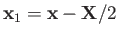 and
and
 , respectively.
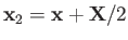
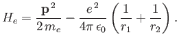
The Hamiltonian of the system is written
, respectively.
The Hamiltonian of the system is written
 |
(9.97) |
where  is the electron momentum,
 ,
,
 , and
, and
 .
Here, we are treating the
protons as essentially stationary, which is a reasonable approximation because the electron's
motion is much more rapid than that of the protons. Of course, this is the case because the electron mass is very much less than the proton mass.
Incidentally, the neglect of nuclear motion when calculating the electronic structure of a molecule is known as the Born-Oppenheimer approximation [13].
.
Here, we are treating the
protons as essentially stationary, which is a reasonable approximation because the electron's
motion is much more rapid than that of the protons. Of course, this is the case because the electron mass is very much less than the proton mass.
Incidentally, the neglect of nuclear motion when calculating the electronic structure of a molecule is known as the Born-Oppenheimer approximation [13].
The Hamiltonian (9.98) is manifestly invariant under the transformation
 , which simply
swaps the positions of the two identical protons.
This transformation is equivalent to
, which simply
swaps the positions of the two identical protons.
This transformation is equivalent to
 . If
. If  is the operator that swaps the proton positions then it is clear that
 . (See Exercise 1.) Hence, the eigenvalues of
are
. (See Exercise 1.) Hence, the eigenvalues of
are
 . Furthermore, the fact that the Hamiltonian is invariant under exchange of proton positions implies that
![$ [P_{12}, H]=0$](img3209.png) . (See Section 9.2.) Thus, the eigenkets of the Hamiltonian are simultaneous eigenkets of
. Now, it
is easily shown that the eigenkets of
corresponding to the eigenvalues
are, respectively, even and odd under
the transformation
. (See Exercise 2.)
It follows that the ground-state wavefunction of the
ion has the general form
. (See Section 9.2.) Thus, the eigenkets of the Hamiltonian are simultaneous eigenkets of
. Now, it
is easily shown that the eigenkets of
corresponding to the eigenvalues
are, respectively, even and odd under
the transformation
. (See Exercise 2.)
It follows that the ground-state wavefunction of the
ion has the general form
![$\displaystyle \psi_\pm({\bf x}) = A\left[\psi_0({\bf x}_1) \pm \psi_0({\bf x}_2)\right],$](img3210.png) |
(9.98) |
where  is a complex number.
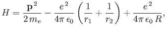
Let us adopt
 |
(9.99) |
as our trial single-proton wavefunction, where
 .
Here,
.
Here,
 is a properly normalized hydrogen ground-state wavefunction, and
  is the Bohr radius.
Thus, our trial molecular wavefunction, which is specified in Equations (9.99) and (9.100), is simply a linear combination of hydrogen ground-state
wavefunctions centered on each proton [18].
is the Bohr radius.
Thus, our trial molecular wavefunction, which is specified in Equations (9.99) and (9.100), is simply a linear combination of hydrogen ground-state
wavefunctions centered on each proton [18].
Our first task is to normalize the trial wavefunction. We require that
 |
(9.100) |
Hence, from Equation (9.99),
 , where
![$\displaystyle I = \int d^{\,3}{\bf x}\left[\vert\psi_0({\bf x}_1)\vert^{\,2} + ...
...psi_0({\bf x}_2)\vert^{\,2} \pm 2\,\psi_0({\bf x}_1)\,\psi_0({\bf x}_2)\right].$](img3215.png) |
(9.101) |
It follows that
 |
(9.102) |
where
 |
(9.103) |
Without loss of generality, we can perform the previous integral using a modified coordinate system in which the
first proton lies at the origin, and the second at
 .
Let
.
Let
 be the position vector of the electron.
It follows that
be the position vector of the electron.
It follows that  and
and
 .
Hence,
.
Hence,
where  and
and  . Here, we have already performed the trivial
  integral.
Let
integral.
Let
 . It follows that
 , giving
Thus,
which evaluates to
 |
(9.107) |
(See Exercise 20.)
Now, the Hamiltonian of the electron is written
 |
(9.108) |
Note, however, that
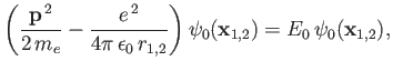 |
(9.109) |
where  is the hydrogen ground-state energy,
because the
is the hydrogen ground-state energy,
because the
 are hydrogen ground-state wavefunctions.
It follows that
are hydrogen ground-state wavefunctions.
It follows that
Hence,
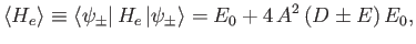 |
(9.111) |
where
Here, use has been made of the fact that
 , as well as the fact that
the Hamiltonian is invariant under the transformation
.
, as well as the fact that
the Hamiltonian is invariant under the transformation
.
Now,
 |
(9.114) |
where
and
,
which reduces to
 |
(9.115) |
giving
![$\displaystyle D = \frac{1}{y} \left[ 1-(1+y)\,{\rm e}^{\,-2\,y}\right].$](img3246.png) |
(9.116) |
(See Exercise 21.)
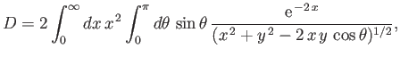
Furthermore,
![$\displaystyle E = 2\int_0^\infty dx\,x\int_0^\pi d\theta\,\sin\theta\,\exp\left[-x-(x^{\,2}+y^{\,2}-2\,x\,y\,\cos\theta)^{1/2}\right],$](img3247.png) |
(9.117) |
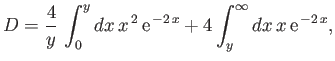
which reduces to
yielding
 |
(9.119) |
(See Exercise 22.)
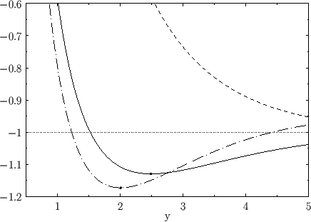
Figure:
The functions  (solid curve) and
  (short-dashed curve), where
. The
long-dash-dotted curve shows the improved
curve obtained from Exercise 23. The dots
indicate the minimum values of
.
(short-dashed curve), where
. The
long-dash-dotted curve shows the improved
curve obtained from Exercise 23. The dots
indicate the minimum values of
.
 |
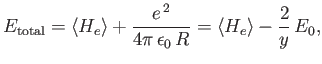
Our final expression for the expectation value of the electron Hamiltonian is
![$\displaystyle \langle H_e\rangle = \left[1+ 2\,\frac{(D\pm E)}{(1\pm J)}\right] E_0,$](img3252.png) |
(9.120) |
where  ,
,  , and
, and  are specified as functions of
in
Equations (9.108), (9.117), and (9.120), respectively.
In order
to obtain the total energy of the molecule, we must add the
potential energy of the two protons to this expectation value. Thus,
are specified as functions of
in
Equations (9.108), (9.117), and (9.120), respectively.
In order
to obtain the total energy of the molecule, we must add the
potential energy of the two protons to this expectation value. Thus,
 |
(9.121) |
because
 .
Hence, we can write
.
Hence, we can write
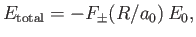 |
(9.122) |
where
![$\displaystyle F_\pm(y) = -1 + \frac{2}{y}\left[\frac{(1+y)\,{\rm e}^{\,-2\,y}\pm(1-2\,y^{\,2}/3) \,{\rm e}^{\,-y}}{1\pm (1+y+y^{\,2}/3)\,{\rm e}^{\,-y}}\right].$](img3255.png) |
(9.123) |
The functions
and
are plotted in Fig. 9.1.
Recall that, in order for the
ion possess a bound state, it must have a lower
energy than a hydrogen atom and a free proton. In other words,
 . It follows, from Equation (9.123), that a bound state
corresponds to
. It follows, from Equation (9.123), that a bound state
corresponds to
 . It is clear, from the figure, that the even trial wavefunction,
  ,
possesses a bound state, whereas the odd trial wavefunction,
,
possesses a bound state, whereas the odd trial wavefunction,  ,
does not. [See Equation (9.99).] This is hardly surprising, because the
even wavefunction maximizes the electron probability density between
the two protons, thereby reducing their mutual electrostatic repulsion. On the other hand, the odd
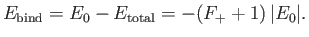
wavefunction does exactly the opposite. The binding energy of the
ion is defined as minus the difference between its energy and that of a
hydrogen atom plus a free proton: that is,
,
does not. [See Equation (9.99).] This is hardly surprising, because the
even wavefunction maximizes the electron probability density between
the two protons, thereby reducing their mutual electrostatic repulsion. On the other hand, the odd
wavefunction does exactly the opposite. The binding energy of the
ion is defined as minus the difference between its energy and that of a
hydrogen atom plus a free proton: that is,
 |
(9.124) |
According to the variational principle, the binding energy is greater than, or
equal to, the maximum binding energy that can be inferred from Figure 9.1. (A maximum in the binding energy
corresponds to a minimum of  .)
This maximum occurs when
.)
This maximum occurs when
 and
and
 .
Thus, our estimates for the equilibrium separation between the two
protons, and the binding energy of the molecule,
are
.
Thus, our estimates for the equilibrium separation between the two
protons, and the binding energy of the molecule,
are
 and
and
 eV, respectively. The experimentally
determined values are
eV, respectively. The experimentally
determined values are
 m, and
 eV, respectively [53]. Clearly, the previous estimates are not particularly accurate. However,
our calculation does establish, beyond any doubt, the existence of
a bound state of the
ion, which is all that we set out to achieve. (See Exercise 23 for a somewhat
improved calculation.)
eV, respectively [53]. Clearly, the previous estimates are not particularly accurate. However,
our calculation does establish, beyond any doubt, the existence of
a bound state of the
ion, which is all that we set out to achieve. (See Exercise 23 for a somewhat
improved calculation.)
We can think of the two constituent protons of the hydrogen molecule ion, whose separation is  , as moving in an electric potential
 due to the combination of their electrostatic repulsion and the binding action of the consistent electron.
Moreover, close to the equilibrium separation,
due to the combination of their electrostatic repulsion and the binding action of the consistent electron.
Moreover, close to the equilibrium separation,  , we have
![$ V(R)\simeq V(R_0) + \left[(1/2)\,F_0''(y_0)/a_0^{\,2}\right]x^{\,2}+ {\cal O}(x^{\,3})$](img3268.png) , where
, where  .
Thus, in the center of mass frame [50], the protons' Hamiltonian takes the form
.
Thus, in the center of mass frame [50], the protons' Hamiltonian takes the form
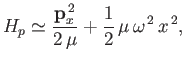 |
(9.125) |
where  is the momentum conjugate to
  ,
,
 the reduced mass [50],
  the proton mass,
 , and we have neglected an unimportant constant term. Here,
  denotes
  . It can be seen, by comparison with Exercise 3,
that the previous Hamiltonian is identical to that of a harmonic oscillator. Thus, the allowed radial oscillation energies of the molecule are
. It can be seen, by comparison with Exercise 3,
that the previous Hamiltonian is identical to that of a harmonic oscillator. Thus, the allowed radial oscillation energies of the molecule are
 |
(9.126) |
where  is a non-negative integer. In particular, there is a non-zero lowest oscillation energy--the so-called zero-point energy [40],
 |
(9.127) |
that must be subtracted from the previously determined electric binding energy of
 to give the true binding energy.
In calculating,
to give the true binding energy.
In calculating,
 we have made use of the numerically determined value
 [derived from Equation (9.124.)]
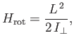
Of course, the hydrogen molecule ion can rotate, as well as vibrate. According to Exercise 7, the rotational
component of the molecular Hamiltonian can be written
 |
(9.128) |
where  is the angular momentum of rotation, and
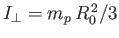 is the molecular moment of inertia [about a perpendicular (to
the line joining the two protons) axis passing through the center of mass].
In calculating the moment of inertia, we have neglected the electron mass, and have treated the protons as point particles. The analysis of Exercise 7
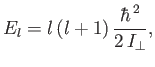
reveals that the rotational energy levels are
is the molecular moment of inertia [about a perpendicular (to
the line joining the two protons) axis passing through the center of mass].
In calculating the moment of inertia, we have neglected the electron mass, and have treated the protons as point particles. The analysis of Exercise 7
reveals that the rotational energy levels are
 |
(9.129) |
where the eigenvalues of  are
are
 , and
, and  is a non-negative integer. It follows that
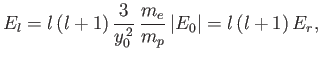
 |
(9.130) |
where
 |
(9.131) |
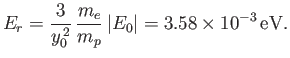
Note that our estimate for the electric binding energy of the hydrogen molecule ion,
, is significantly
greater than our estimate for the zero-point oscillation energy,
 , which, in turn, is very much greater
than a typical rotational energy,
, which, in turn, is very much greater
than a typical rotational energy,
 . This separation in energy scales lies at the heart of
the previously mentioned Born-Oppenheimer approximation [13], according to which the electric, vibrational, and rotational energy levels of molecules
can all be calculated independently of one another.
. This separation in energy scales lies at the heart of
the previously mentioned Born-Oppenheimer approximation [13], according to which the electric, vibrational, and rotational energy levels of molecules
can all be calculated independently of one another.
Next: Exercises
Up: Identical Particles
Previous: Variational Principle
Richard Fitzpatrick
2016-01-22
![$\displaystyle = - \frac{1}{x\,y}\left[{\rm e}^{\,-(x+y)}\,(1+x+y) - {\rm e}^{\,-\vert x-y\vert}\,(1+\vert x-y\vert)\right].$](img3229.png)
![$\displaystyle =A\left[\frac{{\bf p}^{\,2}}{2\,m_e} - \frac{e^{\,2}}{4\pi\,\epsi...
...frac{1}{r_2}\right)\right] \left[\psi_0({\bf x}_1) \pm \psi_0({\bf x}_2)\right]$](img3237.png)
![$\displaystyle = E_0\,\psi_\pm - A\,\left(\frac{e^{\,2}}{4\pi\,\epsilon_0}\right)\left[ \frac{\psi_0({\bf x}_1)}{r_2}\pm \frac{\psi_0({\bf x}_2)}{r_1}\right].$](img3238.png)
![$\displaystyle = 2\int_0^\infty dx\,x^{\,2}\int_0^\pi d\theta\,\sin\theta\,\exp\left[-x-(x^{\,2}+y^{\,2}-2\,x\,y\,\cos\theta)^{1/2}\right],$](img3223.png)
![$\displaystyle = - \frac{2}{y}\,{\rm e}^{\,-y}\int_0^y dx\,x\left[{\rm e}^{\,-2\,x}\,(1+y+x)- (1+y-x)\right]$](img3230.png)
![$\displaystyle \phantom{=}-\frac{2}{y}\int_y^\infty dx\,x\,{\rm e}^{\,-2\,x}\left[{\rm e}^{\,-y}\,(1+y+x)- {\rm e}^{\,y}\,(1-y+x)\right],$](img3231.png)
![$\displaystyle = - \frac{2}{y}\,{\rm e}^{\,-y}\int_0^y dx \left[{\rm e}^{\,-2\,x}\,(1+y+x)- (1+y-x)\right]$](img3248.png)
![$\displaystyle \phantom{=}-\frac{2}{y}\int_y^\infty dx\,{\rm e}^{-2\,x}\left[{\rm e}^{\,-y}\,(1+y+x)- {\rm e}^{\,y}\,(1-y+x)\right],$](img3249.png)