Next: Parallel Wave Propagation Up: Waves in Warm Plasmas Previous: Ion Acoustic Waves Contents
 .
Let us take the perturbed magnetic field into account in our
calculations, in order to allow for
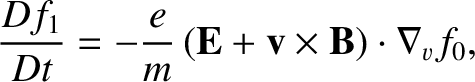
electromagnetic, as well as electrostatic, waves. The linearized Vlasov equation
takes the form
for both ions and electrons, where
.
Let us take the perturbed magnetic field into account in our
calculations, in order to allow for
electromagnetic, as well as electrostatic, waves. The linearized Vlasov equation
takes the form
for both ions and electrons, where  and
and
 are the perturbed electric and magnetic fields, respectively. Likewise,
 is the perturbed distribution function, and
  the equilibrium
distribution function.
the equilibrium
distribution function.
In order to have an equilibrium state at all, we require that
 |
(7.54) |
 , in cylindrical polar coordinates,
 , aligned with the equilibrium magnetic
field, the previous expression can easily be shown to imply that
, aligned with the equilibrium magnetic
field, the previous expression can easily be shown to imply that
 : that is, is a function
only of
: that is, is a function
only of  and
and
 .
.
Let the trajectory of a particle be
 ,
,
 . In the
unperturbed state,
. In the
unperturbed state,
 |
 |
(7.55) |
 |
 |
(7.56) |
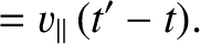
 is the total rate of change of , following the
unperturbed trajectories. Under the assumption that vanishes as
is the total rate of change of , following the
unperturbed trajectories. Under the assumption that vanishes as
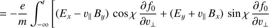
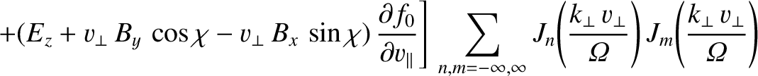
 , the solution to Equation (7.57) can be written
where
, the solution to Equation (7.57) can be written
where  ,
,  is the unperturbed trajectory that passes
through the point
is the unperturbed trajectory that passes
through the point  ,
,  when
when  .
.
It should be noted that the previous method of solution is valid for any set of equilibrium electromagnetic fields, not just a uniform magnetic field. However, in a uniform magnetic field, the unperturbed trajectories are merely helices, whereas in a general field configuration it is difficult to find a closed form for the particle trajectories that is sufficiently simple to allow further progress to be made.
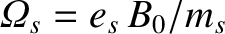
Let us write the velocity in terms of its Cartesian components:
 |
(7.59) |
 is the gyofrequency. The previous
expression can be integrated in time to give
Note that both and
are constants of the motion. This
implies that
is the gyofrequency. The previous
expression can be integrated in time to give
Note that both and
are constants of the motion. This
implies that
 , because is only a
function of and
. Given that
, because is only a
function of and
. Given that
 ,
we can write
,
we can write
Let us assume an
![$\exp[\,{\rm i}\,({\bf k}\cdot{\bf r}-\omega\,t)]$](img1871.png) dependence of all perturbed quantities, with
dependence of all perturbed quantities, with  lying in the
  -
- plane.
Equation (7.58) yields
plane.
Equation (7.58) yields
 |
(7.68) |
 are Bessel functions (Abramowitz and Stegun 1965),
Equation (7.67) gives
where
are Bessel functions (Abramowitz and Stegun 1965),
Equation (7.67) gives
where
 |
(7.70) |
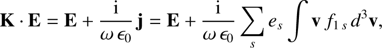
Maxwell's equations yield
 |
 |
(7.71) |
 |
 |
(7.72) |
 is the perturbed current, and
  is the dielectric
permittivity tensor introduced in Section 5.2. It follows that
where
is the dielectric
permittivity tensor introduced in Section 5.2. It follows that
where  is the species-
 perturbed distribution function.
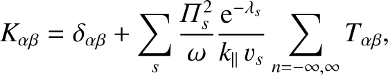
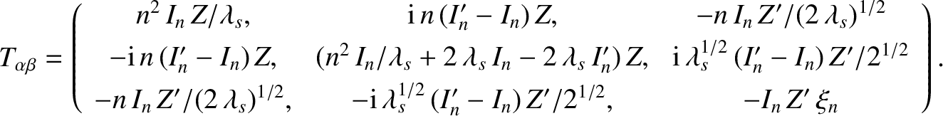
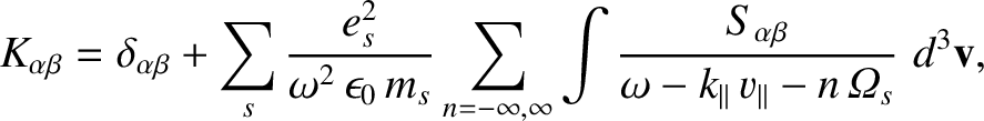
After a great deal of rather tedious analysis, Equations (7.69) and (7.73) reduce to the following expression for the dielectric permittivity tensor (Harris 1970: Cairns 1985):
where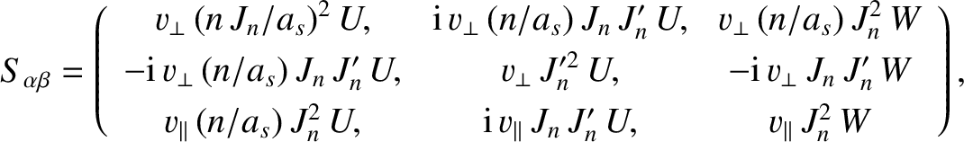 |
(7.75) |
 |
 |
(7.76) |
 |
 |
(7.77) |
 |
 |
(7.78) |
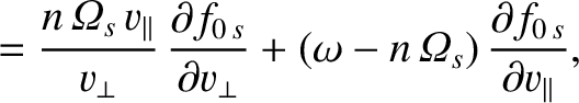
 . In the previous formulae,
  denotes
differentiation with respect to argument, and
denotes
differentiation with respect to argument, and
 .
.
The warm-plasma dielectric tensor, (7.74), can be used to investigate the properties of waves
in just the same manner as the cold-plasma dielectric tensor, (5.37), was employed in
Chapter 5. Note that our expression for the dielectric tensor involves
singular integrals of a type similar to those encountered in Section 7.2. In
principle, this means that we ought to treat the problem as an initial
value problem. Fortunately, we can use the insights gained in our investigation of
the simpler unmagnetized electrostatic wave problem to recognize that the
appropriate way to treat the singular integrals is to evaluate them as
written for
 , and by analytic continuation
for
, and by analytic continuation
for
 .
.
For Maxwellian distribution functions, of the form
we can explicitly perform the velocity-space integral in Equation (7.74), making use of the identities (Watson 1995)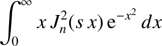 |
 |
(7.80) |
![$\displaystyle \int_0^\infty x^3\left[J_n'(s\,x)\right]^2{\rm e}^{-x^2}\,dx$](img2411.png) |
![$\displaystyle =\frac{1}{4} \,{\rm e}^{-s^2/2}\left[2\,n^2\,I_n(s^2/2)/s^2 + s^2\,I_n(s^2/2)
-s^2\,I_n'(s^2/2)\right],$](img2412.png) |
(7.81) |
 is a modified Bessel function (Abramowitz and Stegun 1965). We obtain
where
is a modified Bessel function (Abramowitz and Stegun 1965). We obtain
where
 ,
,
 , and (Harris 1970; Cairns 1985)
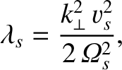
Here,
, and (Harris 1970; Cairns 1985)
Here,  , which is the argument of the modified Bessel functions, is written
whereas
, which is the argument of the modified Bessel functions, is written
whereas  and
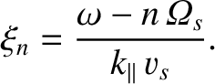
and  represent the plasma dispersion function and its derivative,
both functions being evaluated with the argument
represent the plasma dispersion function and its derivative,
both functions being evaluated with the argument
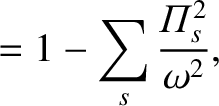
Let us consider the cold-plasma limit,
 . It follows from
Equations (7.84) and (7.85) that this limit corresponds to
. It follows from
Equations (7.84) and (7.85) that this limit corresponds to
 and
and
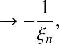
 . According to Equation (7.47),
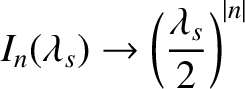
. Moreover, (Abramowitz and Stegun 1965)
as
. It can be demonstrated that the
only non-zero contributions to
 , in this limit, come from
  and
and
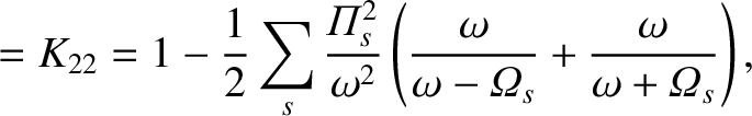
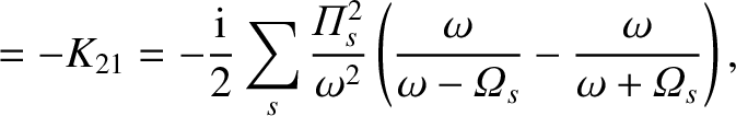
 . In fact,
and
. In fact,
and
 . It is easily seen, from Section 5.3, that the previous
expressions are identical to those found using the cold-plasma fluid
equations. Thus, in the zero temperature limit, the kinetic
dispersion relation obtained in this section reverts to the fluid dispersion
relation derived in Chapter 5.
. It is easily seen, from Section 5.3, that the previous
expressions are identical to those found using the cold-plasma fluid
equations. Thus, in the zero temperature limit, the kinetic
dispersion relation obtained in this section reverts to the fluid dispersion
relation derived in Chapter 5.

![$\displaystyle f_1({\bf r}, {\bf v}, t) =-\frac{e}{m}\int_{-\infty}^t
\left[{\bf...
...+ {\bf v}'\times {\bf B}({\bf r}', t')\right]
\cdot\nabla_v f_0({\bf v}')\,dt',$](img2362.png)
![$\displaystyle {\bf v}' = \left( v_\perp\cos\left[{\mit\Omega}\,(t-t')+\theta\,\...
...\,
v_\perp\sin\left[{\mit\Omega}\,(t-t')+\theta\,\right],\, v_\parallel\right),$](img2369.png)

![$\displaystyle = -\frac{v_\perp}{{\mit\Omega}}\,\left(\sin\left[{\mit\Omega}\,(t-t')
+\theta\,\right] -\sin\theta\right),$](img2372.png)

![$\displaystyle = \frac{v_\perp}{{\mit\Omega}}\,\left(\cos\left[{\mit\Omega}\,(t-t')
+\theta\,\right] -\cos\theta\right),$](img2374.png)


![$\displaystyle = \frac{\partial v_\perp}{\partial v_x'}
\frac{\partial f_0}{\par...
...eft[{\mit\Omega}\,(t'-t)+\theta\,\right]
\frac{\partial f_0}{\partial v_\perp},$](img2380.png)

![$\displaystyle = \frac{\partial v_\perp}{\partial v_y'}
\frac{\partial f_0}{\par...
...eft[{\mit\Omega}\,(t'-t)+\theta\,\right]
\frac{\partial f_0}{\partial v_\perp},$](img2382.png)


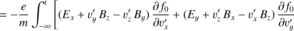
![$\displaystyle \phantom{=}\left.+(E_z + v_x'\,B_y - v_y'\,B_x)\,
\frac{\partial ...
...\left[\,{\rm i}\,\{{\bf k}\cdot
({\bf r}' -{\bf r})-\omega\,(t'-t)\}\right]dt'.$](img2387.png)
![$\displaystyle \phantom{=}\times \exp\left\{\,{\rm i}\left[(n\,{\mit\Omega} + k_\parallel\,v_\parallel-\omega)
\,(t'-t) + (m-n)\,\theta\,\right]\,\right\}dt',$](img2392.png)
![$\displaystyle f_{0\,s} = \frac{n_s}{(2\pi\,T_s/m_s)^{3/2}}\exp\left[-\frac{m_s\,(v_\perp^{2}+v_\parallel^{2})}{2\,T_s}\right],$](img2408.png)