Next: Physics of Landau Damping Up: Waves in Warm Plasmas Previous: Introduction Contents
 ), and possess
a perturbed electric field, but no perturbed magnetic field.
), and possess
a perturbed electric field, but no perturbed magnetic field.
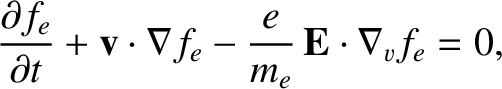
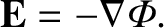
Our starting point is the Vlasov equation for an unmagnetized, collisionless plasma:
where is the ensemble-averaged electron distribution
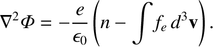
function. The electric field satisfies
where
Here,
is the ensemble-averaged electron distribution
function. The electric field satisfies
where
Here,  is the number density of ions (which is the same
as the equilibrium number density of electrons).
is the number density of ions (which is the same
as the equilibrium number density of electrons).
Because we are dealing with small amplitude waves, it is appropriate to linearize the Vlasov equation. Suppose that the electron distribution function is written
 |
(7.4) |
 represents the equilibrium electron distribution, whereas
  represents the small perturbation due to the wave. Of course,
 , otherwise the equilibrium state would not be quasi-neutral. The electric
field is assumed to be zero in the unperturbed state, so that
, otherwise the equilibrium state would not be quasi-neutral. The electric
field is assumed to be zero in the unperturbed state, so that
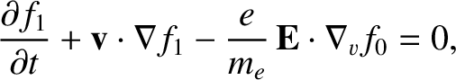
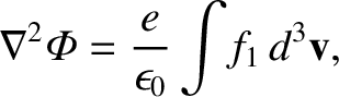
 can be regarded as a small quantity. Thus, linearization of
Equations (7.1) and (7.3) yields
and
respectively.
can be regarded as a small quantity. Thus, linearization of
Equations (7.1) and (7.3) yields
and
respectively.
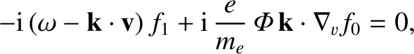
Let us now follow the standard procedure for analyzing small amplitude
waves, by assuming that all perturbed quantities vary with
 and
and  like
like
![$\exp[\,{\rm i}\,({\bf k}\cdot{\bf r}-\omega\,t)]$](img1871.png) .
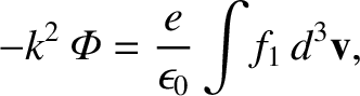
Equations (7.5) and (7.6) reduce to
.
Equations (7.5) and (7.6) reduce to
, and substituting
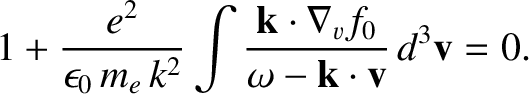
into the integral in the second, we conclude that if
 is non-zero
then we must have
is non-zero
then we must have
We can interpret Equation (7.9) as the dispersion relation for electrostatic plasma
waves, relating the wavevector,  , to the frequency,
  .
However, in doing so, we run up against a serious problem, because the integral has
a singularity in velocity space, where
.
However, in doing so, we run up against a serious problem, because the integral has
a singularity in velocity space, where
 ,
and is, therefore, not properly defined.
,
and is, therefore, not properly defined.
The way to resolve this problem was first explained by Landau in a very
influential paper that was the foundation of much subsequent
work on plasma oscillations and instabilities (Landau 1946). Landau showed that,
instead of simply assuming that varies in time as
 ,
the problem must be regarded as an “initial value problem” in which
is specified at
,
the problem must be regarded as an “initial value problem” in which
is specified at  , and calculated at later times.
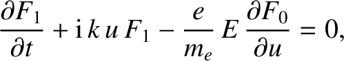
We may still Fourier analyze with respect to , so we write
, and calculated at later times.
We may still Fourier analyze with respect to , so we write
 |
(7.10) |
 as the velocity component along
(i.e.,
as the velocity component along
(i.e.,
 ), and to also define
 and
and  as the integrals of
 and
and
 , respectively, over the velocity components perpendicular to .
Thus, Equations (7.5) and (7.6) yield
and
respectively,
where
, respectively, over the velocity components perpendicular to .
Thus, Equations (7.5) and (7.6) yield
and
respectively,
where
 .
.
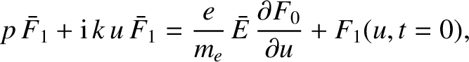
In order to solve Equations (7.11) and (7.12) as an initial value problem, we
introduce the Laplace transform of  with respect to (Riley 1974):
 |
(7.13) |
with increasing is no faster than exponential then the
integral on the right-hand side of the previous equation converges, and defines  as an analytic function of
  , provided
that the real part of is sufficiently large.
, provided
that the real part of is sufficiently large.
Noting that the Laplace transform of
 is
is
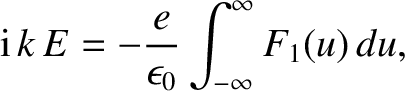
 (as is easily shown by integration by parts), we can Laplace transform Equations (7.11)
and (7.12) to obtain
(as is easily shown by integration by parts), we can Laplace transform Equations (7.11)
and (7.12) to obtain
 |
(7.15) |
![$\displaystyle {\rm i}\,k\,\bar{E} = -\frac{e}{\epsilon_0}\int_{-\infty}^{\infty...
...\partial u}
{p + {\rm i}\,k\,u} + \frac{F_1(u,t=0)}{p+{\rm i}\,k\,u}\right] du,$](img2255.png) |
(7.16) |
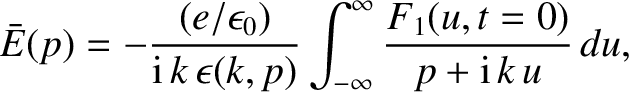
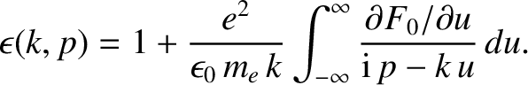
 is known as the plasma dielectric
function. Of course, if is replaced by
is known as the plasma dielectric
function. Of course, if is replaced by
 then
the dielectric function becomes equivalent to the left-hand side
of Equation (7.9). However, because possesses a positive real part, the
integral on the right-hand side of the previous equation is well defined.
then
the dielectric function becomes equivalent to the left-hand side
of Equation (7.9). However, because possesses a positive real part, the
integral on the right-hand side of the previous equation is well defined.
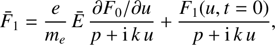
According to Equations (7.14) and (7.17), the Laplace transform of the distribution function is written
 |
(7.19) |
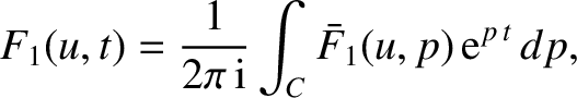
Having found the Laplace transforms of the electric field and the perturbed
distribution function, we must now invert them to obtain
 and as functions of time. The inverse Laplace transform
of the distribution function is given by (Riley 1974)
and as functions of time. The inverse Laplace transform
of the distribution function is given by (Riley 1974)
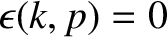
 —the so-called Bromwich contour—is a contour running parallel to
the imaginary axis, and lying to the right of all singularities (otherwise known as poles) of
in the complex- plane. (See Figure 7.1.) There is an analogous
expression for the parallel electric field,
—the so-called Bromwich contour—is a contour running parallel to
the imaginary axis, and lying to the right of all singularities (otherwise known as poles) of
in the complex- plane. (See Figure 7.1.) There is an analogous
expression for the parallel electric field,  .
.
Rather than trying to obtain a general expression for , from
Equations (7.20) and (7.21), we shall concentrate on the behavior of the
perturbed distribution function at large times. Looking at
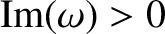
Figure 7.1, we note that if
 has only a finite
number of simple poles in the region
has only a finite
number of simple poles in the region
 (where
  is real and positive) then
we may deform the contour as shown in Figure 7.2, with a loop around
each of the singularities. A pole at
is real and positive) then
we may deform the contour as shown in Figure 7.2, with a loop around
each of the singularities. A pole at  gives a contribution
that varies in time as
gives a contribution
that varies in time as
 , whereas the vertical part of the
contour gives a contribution that varies as
, whereas the vertical part of the
contour gives a contribution that varies as
 . For sufficiently large times,
the latter contribution is negligible, and the behavior is
dominated by contributions from the poles furthest to the right.
. For sufficiently large times,
the latter contribution is negligible, and the behavior is
dominated by contributions from the poles furthest to the right.
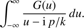
Equations (7.17), (7.18), and (7.20) all involve integrals of the form
Such integrals become singular as approaches the imaginary axis. In order to
distort the contour , in the manner shown in Figure 7.2, we need to continue
these integrals smoothly across the imaginary -axis. As a consequence of the
way in which the Laplace transform was originally defined—that is, for
 sufficiently large—the appropriate way to do this is to take the values
of these integrals when lies in the right-hand half-plane, and to then find the
analytic continuation into the left-hand half-plane (Flanigan 2010).
sufficiently large—the appropriate way to do this is to take the values
of these integrals when lies in the right-hand half-plane, and to then find the
analytic continuation into the left-hand half-plane (Flanigan 2010).
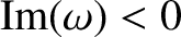
If  is sufficiently well-behaved that it can be continued off the
real axis as an analytic function of a complex variable then the
continuation of (7.22) as the singularity crosses the real axis
in the complex -plane, from the upper to the lower half-plane, is obtained
by letting the singularity take the contour with it, as shown
in Figure 7.3 (Cairns 1985).
is sufficiently well-behaved that it can be continued off the
real axis as an analytic function of a complex variable then the
continuation of (7.22) as the singularity crosses the real axis
in the complex -plane, from the upper to the lower half-plane, is obtained
by letting the singularity take the contour with it, as shown
in Figure 7.3 (Cairns 1985).
Note that the ability to deform the Bromwich contour into that of Figure 7.3, and so to find
a dominant contribution to and
from a few poles, depends on and
 having smooth enough
velocity dependences that the integrals appearing in
Equations (7.17), (7.18), and (7.20) can be analytically continued sufficiently far into the lower
half of the complex -plane (Cairns 1985).
having smooth enough
velocity dependences that the integrals appearing in
Equations (7.17), (7.18), and (7.20) can be analytically continued sufficiently far into the lower
half of the complex -plane (Cairns 1985).
If we consider the electric field given by the inversion of Equation (7.17) then
we see that its behavior at large times is dominated by the zero of
that lies furthest to the right in the complex -plane.
According to Equations (7.20) and (7.21),
has a similar contribution, as well as a contribution that varies in time as
 . Thus, for sufficiently long times after the initial excitation of
the wave, the electric field depends only on the positions of the
roots of
. Thus, for sufficiently long times after the initial excitation of
the wave, the electric field depends only on the positions of the
roots of
 in the complex -plane. The distribution function, on the other hand,
has corresponding components
from these roots, as well as a component that varies in time as
.
At large times, the latter component of the distribution function is
a rapidly oscillating function of velocity, and its contribution to the
charge density, obtained by integrating over , is negligible.
in the complex -plane. The distribution function, on the other hand,
has corresponding components
from these roots, as well as a component that varies in time as
.
At large times, the latter component of the distribution function is
a rapidly oscillating function of velocity, and its contribution to the
charge density, obtained by integrating over , is negligible.
As we have already noted, the function
is equivalent to the
left-hand side of Equation (7.9), provided that is replaced by
.
Thus, the dispersion relation, (7.9), obtained via Fourier transformation of the
Vlasov equation,
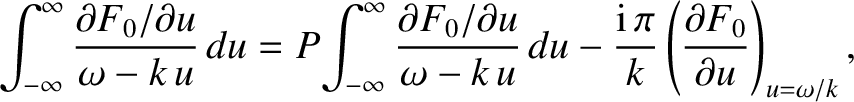
gives the correct behavior at large times, as long as the singular integral
is treated correctly. Adapting the procedure that we discovered using the
complex variable , we see that the integral is defined as it is written for
 , and analytically continued, by deforming the
contour of integration in the -plane (as shown in Figure 7.3), into the region
, and analytically continued, by deforming the
contour of integration in the -plane (as shown in Figure 7.3), into the region
 . The simplest way to remember how to do the
analytic continuation is to observe that the integral is
continued from the part of the -plane corresponding to growing
perturbations to that corresponding to damped perturbations. Once we
know this rule, we can obtain kinetic dispersion relations in a fairly direct manner,
via Fourier
transformation of the Vlasov
equation, and there is no need to attempt the more complicated Laplace transform
solution.
. The simplest way to remember how to do the
analytic continuation is to observe that the integral is
continued from the part of the -plane corresponding to growing
perturbations to that corresponding to damped perturbations. Once we
know this rule, we can obtain kinetic dispersion relations in a fairly direct manner,
via Fourier
transformation of the Vlasov
equation, and there is no need to attempt the more complicated Laplace transform
solution.
In Chapter 5, where we investigated the cold-plasma dispersion relation, we found that
for any given  there were a finite number of values of , say
  ,
,
 ,
,  , and a general solution was a linear superposition of
functions varying in time as
, and a general solution was a linear superposition of
functions varying in time as
 ,
,
 , et cetera. The set of values of corresponding
to a given value of is called the
spectrum of the wave. It is clear that the cold-plasma equations yield a discrete wave spectrum.
On the other hand, in the kinetic problem, we obtain contributions
to the distribution function that vary in time as
,
with taking any real value. In other words, the kinetic equation yields a continuous wave spectrum.
All of the mathematical difficulties of the kinetic
problem arise from the existence of this continuous spectrum (Cairns 1985). At
short times, the behavior is very complicated, and depends on the details
of the initial perturbation. It is only asymptotically that a mode
varying in time as
, et cetera. The set of values of corresponding
to a given value of is called the
spectrum of the wave. It is clear that the cold-plasma equations yield a discrete wave spectrum.
On the other hand, in the kinetic problem, we obtain contributions
to the distribution function that vary in time as
,
with taking any real value. In other words, the kinetic equation yields a continuous wave spectrum.
All of the mathematical difficulties of the kinetic
problem arise from the existence of this continuous spectrum (Cairns 1985). At
short times, the behavior is very complicated, and depends on the details
of the initial perturbation. It is only asymptotically that a mode
varying in time as
 is obtained, with determined
by a dispersion relation that is solely a function of the unperturbed state.
As we have seen, the emergence of such a mode depends on the initial velocity
disturbance being sufficiently smooth.
is obtained, with determined
by a dispersion relation that is solely a function of the unperturbed state.
As we have seen, the emergence of such a mode depends on the initial velocity
disturbance being sufficiently smooth.
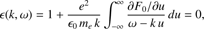
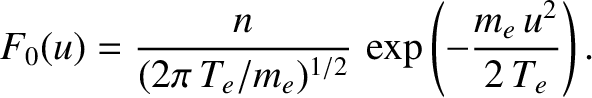
Suppose, for the sake of simplicity, that the background plasma state is a
Maxwellian distribution. Working in terms of , rather than , the kinetic dispersion
relation for electrostatic waves takes the form
is real. Letting
tend to the real axis from the domain
, we obtain
where  denotes the Cauchy principal part of the integral (Flanigan 2010). The origin
of the two terms on the right-hand side of the previous equation is illustrated
in Figure 7.4. The first term—the principal part—is obtained by removing an
interval of length
denotes the Cauchy principal part of the integral (Flanigan 2010). The origin
of the two terms on the right-hand side of the previous equation is illustrated
in Figure 7.4. The first term—the principal part—is obtained by removing an
interval of length
 , symmetrical about the pole,
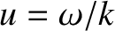 ,
from the range of integration, and then letting
,
from the range of integration, and then letting
 . The
second term comes from the small semi-circle linking the two halves of the
principal part integral. Note that the semi-circle deviates below the
real -axis, rather than above, because the integral is calculated by
letting the pole approach the axis from the upper half-plane
in -space.
. The
second term comes from the small semi-circle linking the two halves of the
principal part integral. Note that the semi-circle deviates below the
real -axis, rather than above, because the integral is calculated by
letting the pole approach the axis from the upper half-plane
in -space.
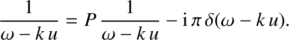
Incidentally, because Equation (7.25) holds for any well-behaved distribution function, it follows that
This famous expression is known as the Plemelj formula (Plemelj 1908).
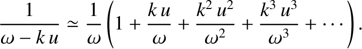
Suppose that is sufficiently small that
 over the
range of where
over the
range of where
 is non-negligible. It follows
that we can expand the denominator of the principal part integral in a
Taylor series:
is non-negligible. It follows
that we can expand the denominator of the principal part integral in a
Taylor series:
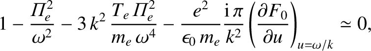
is an odd function, Equation (7.23) reduces to
where
 is the electron plasma frequency.
Equating the real part of the previous expression to zero yields
where
is the electron plasma frequency.
Equating the real part of the previous expression to zero yields
where
 is the Debye length, and it
is assumed that
is the Debye length, and it
is assumed that
 . We can regard the imaginary
part of as a small perturbation, and write
. We can regard the imaginary
part of as a small perturbation, and write
 ,
where
,
where  is the root of Equation (7.29). It follows
that
is the root of Equation (7.29). It follows
that
 |
(7.30) |
If we compare the previous results with those for a cold plasma, where
the dispersion relation for an electrostatic plasma wave was found to
be simply
 (see Section 5.7), we see, first, that now depends on ,
according to Equation (7.29), so that, in a warm plasma, the electrostatic plasma
wave is a propagating mode, with a non-zero group-velocity. Such a mode is known as a Langmuir wave. Second, we
now have
an imaginary part to , given by Equation (7.32), corresponding, because
it is negative, to the damping of the wave in time. This damping is generally
known as Landau damping. If
(i.e.,
if the
wavelength is much larger than the Debye length) then the imaginary part
of is small compared to the real part, and the wave is only
lightly damped. However, as the wavelength becomes comparable to the
Debye length, the imaginary part of becomes comparable to the
real part, and the damping becomes strong.
Admittedly, the approximate solution given previously
is not very accurate in the short wavelength case, but it is nevertheless sufficient to indicate
the existence of very strong damping.
(see Section 5.7), we see, first, that now depends on ,
according to Equation (7.29), so that, in a warm plasma, the electrostatic plasma
wave is a propagating mode, with a non-zero group-velocity. Such a mode is known as a Langmuir wave. Second, we
now have
an imaginary part to , given by Equation (7.32), corresponding, because
it is negative, to the damping of the wave in time. This damping is generally
known as Landau damping. If
(i.e.,
if the
wavelength is much larger than the Debye length) then the imaginary part
of is small compared to the real part, and the wave is only
lightly damped. However, as the wavelength becomes comparable to the
Debye length, the imaginary part of becomes comparable to the
real part, and the damping becomes strong.
Admittedly, the approximate solution given previously
is not very accurate in the short wavelength case, but it is nevertheless sufficient to indicate
the existence of very strong damping.
There are no dissipative effects explicitly included in the collisionless Vlasov equation.
Thus, it can easily be verified that if the particle velocities are
reversed at any time then the solution up to that point is simply reversed in
time. At first sight, this reversible behavior does not seem to be
consistent with the fact that an initial perturbation dies out. However,
we should note that it is only the electric field that decays in time. The
distribution function contains an undamped term varying in time as
. Furthermore, the decay of the electric field depends on there being a
sufficiently smooth initial perturbation in velocity space. The presence
of the
term means that, as time advances, the velocity space dependence of the
perturbation becomes more and more convoluted. It follows that if we
reverse the velocities after some time then we are not starting
with a smooth distribution. Under these circumstances, there is
no contradiction in the fact that, under time reversal, the electric field
grows initially, until the smooth initial state is recreated, and subsequently
decays away (Cairns 1985).
Landau damping was first observed experimentally in the 1960s (Malmberg and Wharton 1964; Malmberg and Wharton 1966; Derfler and Simonen 1966).
![\includegraphics[height=3in]{Chapter07/fig7_1.eps}](img2260.png)

![\includegraphics[height=3in]{Chapter07/fig7_2.eps}](img2269.png)
![\includegraphics[height=2.5in]{Chapter07/fig7_3.eps}](img2273.png)
![\includegraphics[height=2in]{Chapter07/fig7_4.eps}](img2289.png)
![$\displaystyle \omega^2 \simeq {\mit\Pi}_e^{2}\left[1+ 3\,(k\,\lambda_D)^2\right],$](img2295.png)
![$\displaystyle \delta\omega \simeq - {\rm i}\sqrt{\frac{\pi}{8}} \frac{{\mit\Pi}_e}
{(k\,\lambda_D)^3} \exp\left[-\frac{1}{2\,(k\,\lambda_D)^2}\right].$](img2301.png)