Next: Unmagnetized Limit Up: Plasma Fluid Theory Previous: Chapman-Enskog Closure Contents
 , to the
macroscopic lengthscale,
, to the
macroscopic lengthscale,  . This is only appropriate to collisional
plasmas. The second is the ratio of the Larmor radius,
. This is only appropriate to collisional
plasmas. The second is the ratio of the Larmor radius,  , to the macroscopic
lengthscale, . This is only appropriate to magnetized plasmas.
There is, of course, no small parameter upon which to base an asymptotic
closure scheme in a collisionless, unmagnetized plasma. However, such systems
occur predominately in accelerator physics contexts, and are not really
plasmas at all,
because they exhibit virtually no collective effects. Let us
investigate
Chapman-Enskog-like closure schemes
in a collisional, quasi-neutral plasma consisting of
equal numbers of electrons and ions. We shall treat the
unmagnetized and magnetized cases
separately.
, to the macroscopic
lengthscale, . This is only appropriate to magnetized plasmas.
There is, of course, no small parameter upon which to base an asymptotic
closure scheme in a collisionless, unmagnetized plasma. However, such systems
occur predominately in accelerator physics contexts, and are not really
plasmas at all,
because they exhibit virtually no collective effects. Let us
investigate
Chapman-Enskog-like closure schemes
in a collisional, quasi-neutral plasma consisting of
equal numbers of electrons and ions. We shall treat the
unmagnetized and magnetized cases
separately.
The first step in our closure scheme is to approximate the actual collision operator for Coulomb interactions by an operator that is strictly bilinear in its arguments. (See Section 3.10.) Once this has been achieved, the closure problem is formally of the type that can be solved using the Chapman-Enskog method.
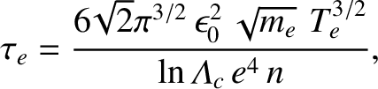
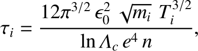
The electron-ion and ion-ion collision times are written
and respectively. (See Section 3.14.) Here, is the number density of particles, and
 is
the Coulomb logarithm, whose origin is the slight modification to the
collision operator mentioned previously. (See Section 3.10.)
is
the Coulomb logarithm, whose origin is the slight modification to the
collision operator mentioned previously. (See Section 3.10.)
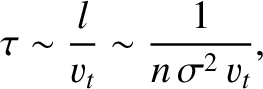
The basic forms of Equations (4.70) and (4.71) are not hard to understand. From Equation (4.58), we expect
 |
(4.72) |
 is the typical “cross-section” of the electrons or ions for
Coulomb “collisions” (i.e., large angle scattering events). Of course, this cross-section is simply the square of
the distance
of closest approach,
is the typical “cross-section” of the electrons or ions for
Coulomb “collisions” (i.e., large angle scattering events). Of course, this cross-section is simply the square of
the distance
of closest approach,  , defined in Equation (1.17). Thus,
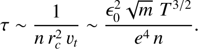 |
(4.73) |
 degree scattering
events) get much longer. It follows that as plasmas are heated they become
less collisional very rapidly.
degree scattering
events) get much longer. It follows that as plasmas are heated they become
less collisional very rapidly.
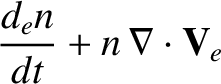
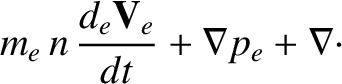
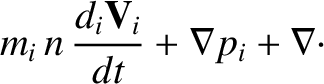
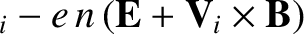
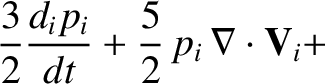
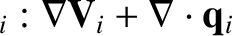
The electron and ion fluid equations in a collisional plasma take the form [see Equations (4.47)–(4.49)]:
and respectively. Here, use has been made of the momentum conservation law, Equation (4.25). Equations (4.74)–(4.76) and (4.77)–(4.79) are called the Braginskii equations, because they were first obtained in a celebrated article by S.I. Braginskii (Braginskii 1965).