In most MHD fluids that occur in astrophysical contexts, the resistivity, ![]() , is extremely
small. Let us consider the perfectly conducting limit,
, is extremely
small. Let us consider the perfectly conducting limit,
![]() .
In this limit, Vainshtein and Zel'dovich introduced an important
distinction
between two fundamentally different classes of dynamo
solution (Vainshtein and Zel'dovich 1972). Suppose that we solve the eigenvalue equation (7.113) to obtain the
growth-rate,
.
In this limit, Vainshtein and Zel'dovich introduced an important
distinction
between two fundamentally different classes of dynamo
solution (Vainshtein and Zel'dovich 1972). Suppose that we solve the eigenvalue equation (7.113) to obtain the
growth-rate, ![]() , of the magnetic field in the limit
, of the magnetic field in the limit
![]() .
We expect that
.
We expect that
| (7.114) |
It is clear, from the discussion in the previous section, that a homopolar disk dynamo is an example of a slow dynamo. In fact, it is easily seen that any dynamo that depends on the motion of a rigid conductor for its operation is bound to be a slow dynamo--in the perfectly conducting limit, the magnetic flux linking the conductor could never change, so there would be no magnetic induction. So, why do we believe that fast dynamo action is even a possibility for an MHD fluid? The answer, of course, is that an MHD fluid is a non-rigid body, and, thus, its motion possesses degrees of freedom not accessible to rigid conductors.
We know that in the perfectly conducting limit (
![]() ) magnetic
field-lines are frozen into an MHD fluid. If the motion is
incompressible (i.e.,
) magnetic
field-lines are frozen into an MHD fluid. If the motion is
incompressible (i.e.,
![]() ) then the stretching
of field-lines implies a proportionate intensification of the field-strength.
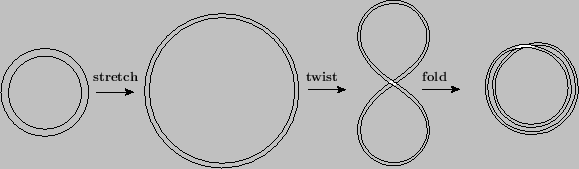
The simplest heuristic fast dynamo, first described by Vainshtein and Zel'dovich,
is based on this effect (Vainshtein and Zel'dovich 1972). As illustrated in Figure 7.6, a magnetic
flux-tube can be doubled in intensity by taking it around a
stretch-twist-fold cycle. The doubling time for this
process clearly does not depend on the resistivity--in this sense, the
dynamo is a fast dynamo. However, under repeated application of the
cycle, the magnetic field develops increasingly fine-scale structure.
In fact, in the limit
) then the stretching
of field-lines implies a proportionate intensification of the field-strength.
The simplest heuristic fast dynamo, first described by Vainshtein and Zel'dovich,
is based on this effect (Vainshtein and Zel'dovich 1972). As illustrated in Figure 7.6, a magnetic
flux-tube can be doubled in intensity by taking it around a
stretch-twist-fold cycle. The doubling time for this
process clearly does not depend on the resistivity--in this sense, the
dynamo is a fast dynamo. However, under repeated application of the
cycle, the magnetic field develops increasingly fine-scale structure.
In fact, in the limit
![]() , both the
, both the ![]() and
and
![]() fields eventually become chaotic and non-differentiable.
A little resistivity is always required to smooth out the fields on
small lengthscales. Even in this case, the fields remain chaotic.
fields eventually become chaotic and non-differentiable.
A little resistivity is always required to smooth out the fields on
small lengthscales. Even in this case, the fields remain chaotic.
At present, the physical existence of fast dynamos has not been
conclusively established, because most of the literature on this
subject is based on mathematical paradigms rather than actual solutions
of the dynamo equation (Childress and Gilbert 1995). It should be noted, however, that the
need for fast dynamo solutions is fairly acute, especially in stellar
dynamo theory. For instance, consider the Sun. The ohmic decay time for the
Sun is about ![]() years, whereas the reversal time for the solar magnetic
field is only 11 years (Mestel 2012). It is obviously a little difficult to believe that resistivity
is playing any significant role in the solar dynamo.
years, whereas the reversal time for the solar magnetic
field is only 11 years (Mestel 2012). It is obviously a little difficult to believe that resistivity
is playing any significant role in the solar dynamo.
In the following, we shall restrict our analysis to slow dynamos, which
undoubtably exist in nature, and which are characterized by non-chaotic
![]() and
and ![]() fields.
fields.