Next: Slow and Fast Dynamos
Up: Magnetohydrodynamic Fluids
Previous: MHD Dynamo Theory
Some of the peculiarities of dynamo theory are well illustrated
by the prototype example of self-excited dynamo action, which is the
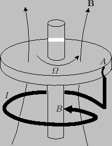
homopolar disk dynamo. As illustrated in Figure 7.5, this device
consists of a conducting disk that rotates at some angular
frequency
 about its axis under the
action of an applied torque. A wire, twisted about the axis in the
manner shown, makes sliding contact with the disc at
about its axis under the
action of an applied torque. A wire, twisted about the axis in the
manner shown, makes sliding contact with the disc at  , and with
the axis at
, and with
the axis at  , and carries a current
  . The magnetic field,
 , associated with this current has a flux
 across the disc, where
  is the mutual inductance between the wire and the
rim of the disc. The rotation of the disc in the
presence of this flux generates a radial electromotive
force
is the mutual inductance between the wire and the
rim of the disc. The rotation of the disc in the
presence of this flux generates a radial electromotive
force
 |
(7.103) |
because a radius of the disc cuts the magnetic flux
 once
every
once
every
 seconds. According to this simplistic
description, the equation for
seconds. According to this simplistic
description, the equation for  is written
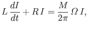 |
(7.104) |
where  is the total resistance of the circuit, and
  is its
self-inductance.
is its
self-inductance.
Figure 7.5:
The homopolar disk dynamo.
 |
Suppose that the angular velocity
is maintained by suitable adjustment
of the driving torque. It follows that Equation (7.104) possesses an
exponential solution
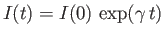 , where
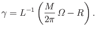 |
(7.105) |
Clearly, we have exponential growth of
--and, hence, of the magnetic
field to which it gives rise (i.e., we have dynamo action)--provided that
 |
(7.106) |
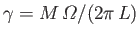
that is, provided that the disk rotates sufficiently rapidly. Note that
the homopolar disk dynamo depends for its success on its built-in
axial asymmetry. If the disk rotates in the opposite
direction to that shown in Figure 7.5, then
 , and the
electromotive force generated by the rotation of the disk always acts
to reduce
. In this case, dynamo action is impossible (i.e.,
, and the
electromotive force generated by the rotation of the disk always acts
to reduce
. In this case, dynamo action is impossible (i.e.,  is always negative). This is a troubling observation,
because most astrophysical objects, such as stars and planets, possess very
good axial symmetry. We conclude that if such bodies are to act
as dynamos then the asymmetry of their internal motions must somehow
compensate for their lack of built-in asymmetry. It is far from obvious
how this is going to happen.
is always negative). This is a troubling observation,
because most astrophysical objects, such as stars and planets, possess very
good axial symmetry. We conclude that if such bodies are to act
as dynamos then the asymmetry of their internal motions must somehow
compensate for their lack of built-in asymmetry. It is far from obvious
how this is going to happen.
Incidentally, although the previous treatment of a homopolar disk dynamo
(which is the standard analysis found in most textbooks) is
very appealing in its simplicity, it cannot be entirely correct.
Consider the limiting situation of a perfectly
conducting disk and wire, in which  . On the one hand,
Equation (7.105) yields
. On the one hand,
Equation (7.105) yields
 , so that
we still have dynamo action. But, on the other hand, the rim of the disk
is a closed circuit embedded in a perfectly conducting medium, so the
flux freezing constraint requires that the flux,
,
through this circuit must remain a constant. There is
an obvious contradiction.
The problem is that we have neglected the currents
that flow azimuthally in the disc: that is, the currents
that control the diffusion of magnetic flux across the rim of
the disk. These currents become particularly important
in the limit
, so that
we still have dynamo action. But, on the other hand, the rim of the disk
is a closed circuit embedded in a perfectly conducting medium, so the
flux freezing constraint requires that the flux,
,
through this circuit must remain a constant. There is
an obvious contradiction.
The problem is that we have neglected the currents
that flow azimuthally in the disc: that is, the currents
that control the diffusion of magnetic flux across the rim of
the disk. These currents become particularly important
in the limit
 .
.
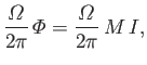
The previous paradox can be resolved by supposing that the azimuthal current,
 , is constrained to flow around the rim of the disk (e.g.,
by a suitable distribution of radial insulating strips). In this
case, the fluxes through the
and
, is constrained to flow around the rim of the disk (e.g.,
by a suitable distribution of radial insulating strips). In this
case, the fluxes through the
and  circuits are
and the equations governing the current flow become
where  , and
, and  refer to the
circuit. Let us search
for exponential solutions,
refer to the
circuit. Let us search
for exponential solutions,
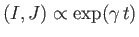 , of the
previous system of equations. It is easily
demonstrated that
, of the
previous system of equations. It is easily
demonstrated that
 |
(7.111) |
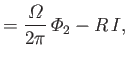
Recall the standard result in electromagnetic theory that
 for two
non-coincident circuits (Jackson 1998). It is clear, from the previous expression, that the
condition for dynamo action (i.e.,
for two
non-coincident circuits (Jackson 1998). It is clear, from the previous expression, that the
condition for dynamo action (i.e.,  ) is
) is
 |
(7.112) |
as before. Note, however, that
 as
as
 .
In other words, if the rotating disk is a perfect conductor then dynamo
action is impossible. The previous system of equations can be transformed
into the well-known Lorenz system, which exhibits chaotic behavior
in certain parameter regimes (Knobloch 1981). It is noteworthy that this simplest prototype
dynamo system already contains the seeds of chaos (provided that
the formulation is self-consistent).
.
In other words, if the rotating disk is a perfect conductor then dynamo
action is impossible. The previous system of equations can be transformed
into the well-known Lorenz system, which exhibits chaotic behavior
in certain parameter regimes (Knobloch 1981). It is noteworthy that this simplest prototype
dynamo system already contains the seeds of chaos (provided that
the formulation is self-consistent).
The previous discussion implies that, while dynamo action requires the
resistance,
, of the circuit to be low, we lose dynamo action
altogether if we go to the
perfectly conducting limit,
 , because magnetic fields are unable to diffuse
into the region in which magnetic induction is operating. Thus, an efficient
dynamo requires a conductivity that is large, but not too large.
, because magnetic fields are unable to diffuse
into the region in which magnetic induction is operating. Thus, an efficient
dynamo requires a conductivity that is large, but not too large.
Next: Slow and Fast Dynamos
Up: Magnetohydrodynamic Fluids
Previous: MHD Dynamo Theory
Richard Fitzpatrick
2016-01-23