


Next: Method of Stationary Phase
Up: Wave Propagation in Uniform
Previous: Wave-Front Propagation
Sommerfeld Precursor
Consider the situation immediately after the arrival of the
signal: that is, when  is small and positive. Let us start from
Equation (887), which can be written in the form
is small and positive. Let us start from
Equation (887), which can be written in the form
![$\displaystyle f(x,t) = \frac{1}{\tau}\int_C {\rm e}^{\,{\rm i}\,([k-\omega/c]\,x-\omega\, s)} \frac{d\omega}{\omega^{\,2} -(2\pi/\tau)^{\,2}}.$](img1853.png) |
(890) |
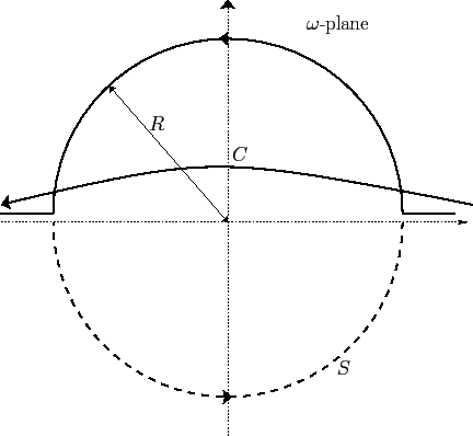
We can deform the original path of integration  into a large semi-circle
of radius
into a large semi-circle
of radius  in the upper half-plane, plus two segments of the real axis,
as shown in Figure 9. Because of the denominator
in the upper half-plane, plus two segments of the real axis,
as shown in Figure 9. Because of the denominator
 ,
the integrand tends to zero as
,
the integrand tends to zero as
 on the real axis. We can add the
path in the lower half-plane that is shown as a dotted line in the figure,
because if the radius of the semi-circular portion of this lower path
is increased to infinity then the integrand vanishes exponentially
as
on the real axis. We can add the
path in the lower half-plane that is shown as a dotted line in the figure,
because if the radius of the semi-circular portion of this lower path
is increased to infinity then the integrand vanishes exponentially
as  . Therefore, we can replace our original path of integration
by the entire circle
. Therefore, we can replace our original path of integration
by the entire circle  . Thus,
![$\displaystyle f(x,t) = \frac{1}{\tau}\oint_S{\rm e}^{\,{\rm i}\,([k-\omega/c]\,x-\omega\, s)} \frac{d\omega}{\omega^{\,2} -(2\pi/\tau)^{\,2}}$](img1855.png) |
(891) |
in the limit that the radius of the circle
tends to infinity.
Figure 9:
Sketch of the integration contour used to evaluate Equation (891).
 |
The dispersion relation (871) yields
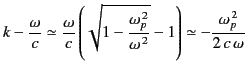 |
(892) |
in the limit
 . Using the abbreviation
 |
(893) |
and, henceforth, neglecting  with respect to
  , we
obtain
, we
obtain
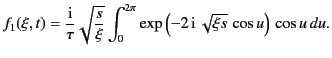
![$\displaystyle f(x,t) = f_1(\xi,t) \simeq\frac{1}{\tau} \oint_S \exp\left[\,{\rm...
...eft( -\frac{\xi}{\omega} -\omega\, s\right)\right]\frac{d\omega} {\omega^{\,2}}$](img1860.png) |
(894) |
from Equation (892).
This expression can also be written
![$\displaystyle f_1(\xi,t) = \frac{1}{\tau} \oint_S \exp\left[\,-{\rm i}\, \sqrt{...
...xi}{s}}+\omega \sqrt{\frac{s}{\xi}}\right)\right] \frac{d\omega}{\omega^{\,2}}.$](img1861.png) |
(895) |
Let
 |
(896) |
It follows that
 |
(897) |
giving
 |
(898) |
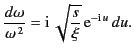
Substituting the
angular variable  for
in Equation (896), we obtain
for
in Equation (896), we obtain
 |
(899) |
Here, we have taken
 as the radius of the circular
integration path in the
-plane. This is indeed a large radius
because
as the radius of the circular
integration path in the
-plane. This is indeed a large radius
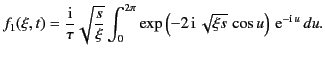
because  . From symmetry, Equation (900) simplifies to give
 |
(900) |
The following mathematical identity is fairly well known,![[*]](footnote.png)
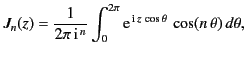 |
(901) |
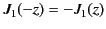
where
 is Bessel function of order
  . It follows from Equation (901)
that
. It follows from Equation (901)
that
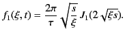 |
(902) |
Here, we have made use of the fact that
 .
.
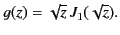
Figure:
The Bessel function  .
.
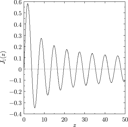 |
The properties of Bessel functions are described in many
standard references on mathematical functions (see, for instance,
Abramowitz and Stegun). In the small argument limit,
 , we find that
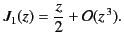 |
(903) |
On the other hand, in the large argument limit,  , we obtain
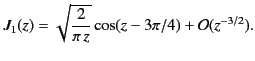 |
(904) |
The behavior of
is further illustrated in Figure 10.
We are now in a position to make some quantitative statements regarding
the signal that first arrives at a depth  within the dispersive medium.
This signal propagates at the velocity of light in vacuum, and
is called the Sommerfeld precursor. The first important point
to note is that the amplitude of the Sommerfeld precursor is very small
compared to that of the incident wave (whose amplitude is normalized to
unity). We can easily see this because, in deriving Equation (903),
we assumed that
within the dispersive medium.
This signal propagates at the velocity of light in vacuum, and
is called the Sommerfeld precursor. The first important point
to note is that the amplitude of the Sommerfeld precursor is very small
compared to that of the incident wave (whose amplitude is normalized to
unity). We can easily see this because, in deriving Equation (903),
we assumed that
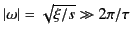 on the circular integration
path
. Because the magnitude of
on the circular integration
path
. Because the magnitude of  is always less than, or of order,
unity, it is clear that
is always less than, or of order,
unity, it is clear that
 . This is a comforting result, because
in a naive treatment of wave propagation through a dielectric medium, the
wave-front propagates at the group velocity
. This is a comforting result, because
in a naive treatment of wave propagation through a dielectric medium, the
wave-front propagates at the group velocity  (which is less
than
(which is less
than  ) and, therefore, no signal should reach a depth
within the medium
before time
) and, therefore, no signal should reach a depth
within the medium
before time  . We are finding that there is, in fact, a precursor
that arrives at
. We are finding that there is, in fact, a precursor
that arrives at  , but that this signal is fairly weak. Note
from Equation (894) that
, but that this signal is fairly weak. Note
from Equation (894) that  is proportional to
. Consequently, the
amplitude of the Sommerfeld precursor decreases as the inverse of the
distance traveled by the wave-front through the dispersive medium
[because
is proportional to
. Consequently, the
amplitude of the Sommerfeld precursor decreases as the inverse of the
distance traveled by the wave-front through the dispersive medium
[because
 attains its maximum value when
 ].
Thus, the Sommerfeld precursor is likely to become undetectable after
the wave has traveled a long distance through the medium.
].
Thus, the Sommerfeld precursor is likely to become undetectable after
the wave has traveled a long distance through the medium.
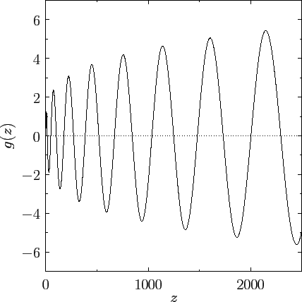
Figure 11:
The Sommerfeld precursor.
 |
Equation (903) can be written
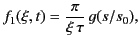 |
(905) |
where
 , and
, and
 |
(906) |
The normalized Sommerfeld precursor  is shown in Figure 11. It
can be seen that both the amplitude and the oscillation period
of the precursor gradually increase. The roots of
[i.e.,
the solutions of
is shown in Figure 11. It
can be seen that both the amplitude and the oscillation period
of the precursor gradually increase. The roots of
[i.e.,
the solutions of  ] are spaced at distances of approximately
 apart. Thus, the time interval for the
  th half period of the
precursor is approximately given by
th half period of the
precursor is approximately given by
 |
(907) |
Note that the initial period of oscillation,
 |
(908) |
is extremely small compared to the incident period  . Moreover,
the initial period of oscillation is completely independent of the
frequency of the incident wave. In fact,
. Moreover,
the initial period of oscillation is completely independent of the
frequency of the incident wave. In fact,
 depends only
on the propagation distance
, and the dispersive power of the medium. The
period also decreases with increasing distance,
, traveled by the wave-front though the medium. So, when visible radiation is incident on
a dispersive medium, it is quite possible for the first signal
detected well inside the medium to lie in the X-ray region of the
electromagnetic spectrum.
depends only
on the propagation distance
, and the dispersive power of the medium. The
period also decreases with increasing distance,
, traveled by the wave-front though the medium. So, when visible radiation is incident on
a dispersive medium, it is quite possible for the first signal
detected well inside the medium to lie in the X-ray region of the
electromagnetic spectrum.
Next: Method of Stationary Phase
Up: Wave Propagation in Uniform
Previous: Wave-Front Propagation
Richard Fitzpatrick
2014-06-27