Properties of Multipole Fields

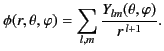
Let us examine some of the properties of the multipole fields (1470)-(1471) and (1474)-(1475). Consider, first of all, the so-called near zone, in which $k\,r\ll 1$ . In this region, $f_l(k\,r)$ is dominated by $y_l(k\,r)$ , which blows up as $k\,r\rightarrow 0$ , and which has the asymptotic expansion (1429), unless the coefficient of $y_l(k\,r)$ vanishes identically. Excluding this possibility, the limiting behavior of the magnetic field for an electric $l, m$ multipole is

$$c\,{\bf B}_{lm}^{(E)} \rightarrow -\frac{k}{l}\, {\bf L} \,\frac{Y_{lm}}{r^{\,l+1}},$$ (1483)

where the proportionality constant is chosen for later convenience. To find the corresponding electric field, we must take the curl of the right-hand side of the above equation. The following operator identity is useful

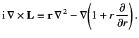$${\rm i}\,\nabla\times{\bf L} \equiv {\bf r}\,\nabla^{\,2} -\nabla\!\left( 1+ r\,\frac{\partial}{\partial r}\right).$$ (1484)

The electric field (1475) can be written

$${\bf E}_{lm}^{(E)} \rightarrow \frac{-{\rm i}}{l}\,\nabla\times {\bf L} \left(\frac{Y_{lm}}{r^{\,l+1}}\right).$$ (1485)

Because $Y_{lm}/r^{\,l+1}$ is a solution of Laplace's equation, it is annihilated by the first term on the right-hand side of (1486). Consequently, for an electric $l, m$ multipole, the electric field in the near zone becomes

$${\bf E}_{lm}^{(E)} \rightarrow -\nabla\left(\frac{Y_{lm}}{r^{\,l+1}}\right).$$ (1486)

This, of course, is an electrostatic multipole field. Such a field can be obtained in a more straightforward manner by observing that ${\bf E}\rightarrow -\nabla\phi$ , where $\nabla^{\,2}\phi = 0$ , in the near zone. Solving Laplace's equation by separation of variables in spherical coordinates, and demanding that $\phi$ be well behaved as $\vert{\bf r}\vert\rightarrow\infty$ , yields

$$\phi(r,\theta,\varphi) = \sum_{l,m}\frac{Y_{lm}(\theta,\varphi)}{r^{\,l+1}}.$$ (1487)

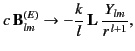
Note that ($c$ times) the magnetic field (1485) is smaller than the electric field (1488) by a factor of order $k\,r$ . Thus, in the near zone, ($c$ times) the magnetic field associated with an electric multipole is much smaller than the corresponding electric field. For magnetic multipole fields, it is evident from Equations (1470)-(1471) and (1474)-(1475) that the roles of ${\bf E}$ and $c\,{\bf B}$ are interchanged according to the transformation

$${\bf E}^{(E)} \rightarrow -c\,{\bf B}^{(M)},$$ (1488)

$$c\,{\bf B}^{(E)} \rightarrow {\bf E}^{(M)}.$$ (1489)

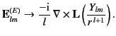
In the so-called far zone, or radiation zone, in which $k\,r\gg 1$ , the multipole fields depend on the boundary conditions imposed at infinity. For definiteness, let us consider the case of outgoing waves at infinity, which is appropriate to radiation by a localized source. For this case, the radial function $f_l(k\,r)$ contains only the spherical Hankel function $h_l^{(1)}(k\,r)$ . From the asymptotic form (1432), it is clear that in the radiation zone the magnetic field of an electric $l, m$ multipole varies as

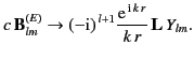$$c\,{\bf B}_{lm}^{(E)} \rightarrow (-{\rm i})^{\,l+1} \frac{{\rm e}^{\,{\rm i}\,k\,r}} {k\,r}\, {\bf L} \,Y_{lm}.$$ (1490)

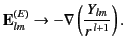
Using Equation (1475), the corresponding electric field can be written

$${\bf E}_{lm}^{(E)} = \frac{(-{\rm i})^{\,l}}{k^{\,2}}\left[\nabla... ...} +\frac{{\rm e}^{\,{\rm i}\,k\,r}}{r} \,\nabla\times {\bf L} \,Y_{lm} \right].$$ (1491)

Neglecting terms that fall off faster than $1/r$ , the above expression reduces to

$${\bf E}_{lm}^{(E)} = -(-{\rm i})^{\,l+1} \frac{{\rm e}^{\,{\rm i}... ...\times {\bf L}\,Y_{lm}-\frac{1}{k}({\bf r}\,\nabla^{\,2}-\nabla) Y_{lm}\right],$$ (1492)

where use has been made of the identity (1486), and ${\bf n} = {\bf r}/r$ is a unit vector pointing in the radial direction. The second term in square brackets is smaller than the first term by a factor of order $1/(k\,r)$ , and can, therefore, be neglected in the limit $k\,r\gg 1$ . Thus, we find that the electric field in the radiation zone takes the form

$${\bf E}_{lm}^{(E)} = c\,{\bf B}_{lm}^{(E)}\times{\bf n},$$ (1493)

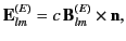
where $c\,{\bf B}_{lm}^{(E)}$ is given by Equation (1492). These fields are typical radiation fields: that is, they are transverse to the radius vector, mutually orthogonal, fall off like $1/r$ , and are such that $\vert{\bf E}\vert=c\,\vert{\bf B}\vert$ . To obtain expansions for magnetic multipoles, we merely make the transformation (1490)-(1491).

Consider a linear superposition of electric $l, m$ multipoles with different $m$ values that all possess a common $l$ value. Suppose that all multipoles correspond to outgoing waves at infinity. It follows from Equations (1474)-(1476) that

$$c\,{\bf B}_l = \sum_l a_E(l,m) \, h_l^{(1)}(k\,r)\,{\rm e}^{-{\rm i}{ \,\omega \,t}}\,{\bf X}_{lm},$$ (1494)

$${\bf E}_l = \frac{\rm i}{k}\,\nabla\times c\, {\bf B}_{l}.$$ (1495)

For harmonically varying fields, the time-averaged energy density is given by

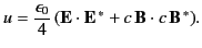$$u = \frac{\epsilon_0}{4}\,({\bf E}\cdot{\bf E}^{\,\ast} + c\,{\bf B}\cdot c\,{\bf B}^{\,\ast}).$$ (1496)

In the radiation zone, the two terms on the right-hand side of the above equation are equal. It follows that the energy contained in a spherical shell lying between radii $r$ and $r+dr$ is

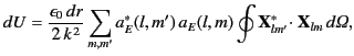$$dU = \frac{\epsilon_0\,dr}{2\,k^{\,2}}\sum_{m,m'} a_E^\ast(l,m') \,a_E(l,m) \oint {\bf X}_{lm'}^\ast\!\cdot{\bf X}_{lm} \,d{\mit\Omega},$$ (1497)

where use has been made of the asymptotic form (1432) of the spherical Hankel function $h_l^{(1)}(z)$ . The orthogonality relation (1477) leads to

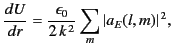$$\frac{dU}{dr} = \frac{\epsilon_0}{2\,k^{\,2}} \sum_m \vert a_E(l,m)\vert^{\,2},$$ (1498)

which is clearly independent of the radius. For a general superposition of electric and magnetic multipoles, the sum over $m$ becomes a sum over $l$ and $m$ , whereas $\vert a_E\vert^{\,2}$ becomes $\vert a_E\vert^{\,2}+\vert a_M\vert^{\,2}$ . Thus, the net energy in a spherical shell situated in the radiation zone is an incoherent sum over all multipoles.

The time-averaged angular momentum density of harmonically varying electromagnetic fields is given by

$${\bf m} = \frac{\epsilon_0}{2}\, {\rm Re}\, [{\bf r}\times({\bf E}\times {\bf B}^{\,\ast})].$$ (1499)

For a superposition of electric multipoles, the triple product can be expanded, and the electric field (1497) substituted, to give

$${\bf m} = \frac{\epsilon_0 \,c}{2\,k} \,{\rm Re}\,[{\bf B}^{\,\ast}({\bf L}\cdot {\bf B})].$$ (1500)

Thus, the net angular momentum contained in a spherical shell lying between radii $r$ and $r+dr$ (in the radiation zone) is

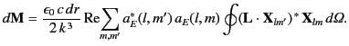$$d{\bf M} = \frac{\epsilon_0\, c \,dr} {2\,k^{\,3}} \,{\rm Re} \!\... ...l,m) \oint ({\bf L}\cdot{\bf X}_{lm'})^{\,\ast}\, {\bf X}_{lm} \,d{\mit\Omega}.$$ (1501)

It follows from Equations (1436) and (1476) that

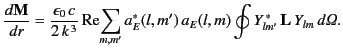$$\frac{d{\bf M}}{dr} = \frac{\epsilon_0 \,c}{2\,k^{\,3}} \,{\rm Re... ..._E^\ast(l,m')\,a_E(l,m) \oint Y_{lm'}^{\,\ast}\,{\bf L}\,Y_{lm}\,d{\mit\Omega}.$$ (1502)

According to Equations (1439)-(1441), the Cartesian components of $d{\bf M}/dr$ can be written:

$$\frac{d M_x}{dr} =\frac{\epsilon_0 \,c}{4\, k^{\,3}} \,{\rm Re}\!\sum_m\left[\sqrt{(l-m)\,(l+m+1)}\, a_E^{\,\ast}(l, m+1)\right.$$

$$\left.+ \sqrt{(l+m)\,(l-m+1)} \,a_E^{\,\ast}(l,m-1)\right]a_E(l,m),$$ (1503)

$$\frac{d M_y}{dr} = \frac{\epsilon_0 \,c}{4 \,k^{\,3}} \,{\rm Im}\!\sum_m\left[\sqrt{(l-m)\,(l+m+1)}\, a_E^{\,\ast}(l, m+1)\right.$$

$$\left. - \sqrt{(l+m)\,(l-m+1)} \,a_E^{\,\ast}(l,m-1)\right]a_E(l,m),$$ (1504)

$$\frac{d M_z}{dr} = \frac{\epsilon_0 \,c}{2 \,k^{\,3}} \sum_m m\,\vert a_E(l,m)\vert^{\,2}.$$ (1505)

Thus, for a general $l$ th order electric multipole that consists of a superposition of different $m$ values, only the $z$ component of the angular momentum takes a relatively simple form.