Next: Angular Momentum Operators
Up: Multipole Expansion
Previous: Introduction
Multipole Expansion of Scalar Wave Equation
Before considering the vector wave equation, let us
consider the somewhat simpler
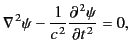
scalar wave equation. A scalar field
 satisfying the homogeneous wave equation,
 |
(1409) |
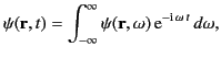
can be Fourier analyzed in time,
 |
(1410) |
with each Fourier harmonic satisfying the homogeneous Helmholtz wave equation,
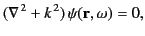 |
(1411) |
where
 . We can write the Helmholtz equation in
terms of spherical coordinates
. We can write the Helmholtz equation in
terms of spherical coordinates  ,
,  ,
,  :
:
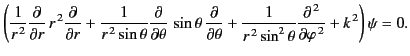 |
(1412) |
As is well known, it is possible to solve this equation via
separation of variables to give
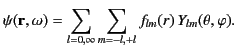 |
(1413) |
Here, we restrict our attention to physical
solutions that are well-behaved in the angular variables
and
.
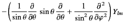
The spherical harmonics
 satisfy
the following equations:
satisfy
the following equations:
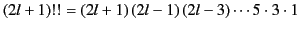
where  is a non-negative integer, and
  is an integer that
satisfies the inequality
is an integer that
satisfies the inequality  . The radial functions
 satisfy
![$\displaystyle \left[\frac{d^{\,2}}{dr^{\,2}} + \frac{2}{r}\frac{d}{dr} + k^{\,2} - \frac{l\,(l+1)}{r^{\,2}} \right]f_{lm}(r) =0.$](img3008.png) |
(1416) |
With the substitution
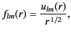 |
(1417) |
Equation (1418) is transformed into
![$\displaystyle \left[\frac{d^{\,2}}{dr^{\,2}} + \frac{1}{r}\frac{d}{dr} +k^{\,2} - \frac{(l+1/2)^{\,2}}{r^{\,2}}\right] u_{lm}(r) =0,$](img3010.png) |
(1418) |
which is a type of
Bessel equation of half-integer order,  . Thus, we can write
the solution for
as
. Thus, we can write
the solution for
as
 |
(1419) |
where  and
and  are arbitrary constants.
The half-integer order Bessel functions
are arbitrary constants.
The half-integer order Bessel functions
 and
and
 have analogous properties to the integer order
Bessel functions
have analogous properties to the integer order
Bessel functions  and
and  . In particular,
the
are well behaved in the limit
. In particular,
the
are well behaved in the limit
 ,
whereas the
are badly behaved.
,
whereas the
are badly behaved.
It is convenient to define the spherical Bessel functions,
 and
and  , where
It is also convenient to define the spherical Hankel functions,
 and
and
 , where
Assuming that  is real,
 is the complex conjugate of
 .
It turns out that
the spherical Bessel functions can be expressed
in the closed form
.
It turns out that
the spherical Bessel functions can be expressed
in the closed form
In the limit of small argument,
where
 .
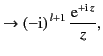
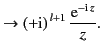
In the limit of large argument,
.
In the limit of large argument,
which implies that
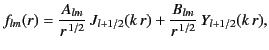
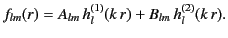
It follows, from the above discussion, that the radial functions
, specified in Equation (1421),
can also be written
 |
(1432) |
Hence, the general solution of the homogeneous Helmholtz equation, (1413), takes the form
![$\displaystyle \psi({\bf r},\omega) = \sum_{l=0,\infty}\sum_{m=-l,+l}\left[A_{lm}\,h_l^{(1)}(k\,r) + B_{lm}\,h_l^{(2)}(k\,r)\right]Y_{lm}(\theta,\varphi).$](img3042.png) |
(1433) |
Moreover, it is clear from Equations (1412) and (1432)-(1433) that, at large
, the terms involving the
 Hankel functions correspond
to outgoing radial waves, whereas those involving the
Hankel functions correspond
to outgoing radial waves, whereas those involving the
 functions correspond to incoming radial waves.
Next: Angular Momentum Operators
Up: Multipole Expansion
Previous: Introduction
Richard Fitzpatrick
2014-06-27

![$\displaystyle \rightarrow \frac{z^{\,l}}{(2\,l+1)!!}\left[1+ {\cal O}(z^2)\right],$](img3034.png)
![$\displaystyle \rightarrow -\frac{(2\,l-1)!!}{z^{\,l+1}}\left[1+ {\cal O}(z^2)\right],$](img3035.png)