


Next: Electromagnetic energy and momentum
Up: Magnetic induction
Previous: Alternating current circuits
Transmission lines
The central assumption made in the analysis of conventional AC circuits is that
the voltage (and, hence, the current) has the same phase throughout the circuit.
Unfortunately, if the circuit is sufficiently large, or the frequency of
oscillation,  , is sufficiently high, then this assumption becomes invalid.
The assumption of a constant phase throughout the circuit is reasonable if the
wave-length of the oscillation,
, is sufficiently high, then this assumption becomes invalid.
The assumption of a constant phase throughout the circuit is reasonable if the
wave-length of the oscillation,
 , is
much larger than the dimensions of
the circuit. (Here, we assume that signals propagate around electrical circuits
at about the velocity of light. This assumption will be justified later on.)
This is generally not the case in electrical circuits which are
associated with communication. The frequencies in such
circuits tend to be very high, and the dimensions are, almost
by definition, large. For instance,
leased telephone lines (the type you attach computers to) run at
, is
much larger than the dimensions of
the circuit. (Here, we assume that signals propagate around electrical circuits
at about the velocity of light. This assumption will be justified later on.)
This is generally not the case in electrical circuits which are
associated with communication. The frequencies in such
circuits tend to be very high, and the dimensions are, almost
by definition, large. For instance,
leased telephone lines (the type you attach computers to) run at
 kHz. The corresponding wave-length is about 5 km, so the constant-phase
approximation clearly breaks down for long-distance calls. Computer networks
generally run at about 100 MHz, corresponding to
kHz. The corresponding wave-length is about 5 km, so the constant-phase
approximation clearly breaks down for long-distance calls. Computer networks
generally run at about 100 MHz, corresponding to
 m. Thus,
the constant-phase approximation also breaks down for most computer networks,
since such networks are generally significantly larger than 3m.
It turns out that you need a
special sort of wire, called a transmission line, to propagate signals around circuits
whose dimensions greatly exceed the wave-length,
m. Thus,
the constant-phase approximation also breaks down for most computer networks,
since such networks are generally significantly larger than 3m.
It turns out that you need a
special sort of wire, called a transmission line, to propagate signals around circuits
whose dimensions greatly exceed the wave-length,  . Let us investigate
transmission lines.
. Let us investigate
transmission lines.
An idealized transmission line consists of two parallel conductors of uniform
cross-sectional area.
The conductors possess a capacitance per unit length,
 , and an inductance per unit length,
  . Suppose that
  measures the position
along the line.
measures the position
along the line.
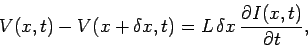
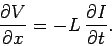
Consider the voltage difference between two neighbouring points
on the line, located at positions and  , respectively.
The self-inductance of the portion of the line lying between these two
points is
, respectively.
The self-inductance of the portion of the line lying between these two
points is  . This small section of the line can be thought of as
a conventional inductor, and, therefore, obeys the well-known equation
. This small section of the line can be thought of as
a conventional inductor, and, therefore, obeys the well-known equation
 |
(990) |
where  is the voltage difference between the two conductors at
position and time
is the voltage difference between the two conductors at
position and time  , and
, and
 is the current flowing in one of the conductors at position
and time [the current flowing
in the other conductor is
is the current flowing in one of the conductors at position
and time [the current flowing
in the other conductor is  ]. In the limit
 ,
the above equation reduces to
,
the above equation reduces to
 |
(991) |
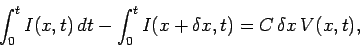
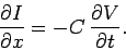
Consider the difference in current between two neighbouring points on the
line, located at positions and , respectively. The capacitance
of the portion of the line lying between these two points is
 . This small section of the line can be thought of
as a conventional capacitor, and, therefore, obeys the well-known equation
. This small section of the line can be thought of
as a conventional capacitor, and, therefore, obeys the well-known equation
 |
(992) |
where  denotes a time at which the charge stored in either of
the conductors in the region to
is zero. In the limit
, the above equation
yields
denotes a time at which the charge stored in either of
the conductors in the region to
is zero. In the limit
, the above equation
yields
 |
(993) |
Equations (991) and (993) are generally known as the telegrapher's equations,
since an old fashioned telegraph line can be thought of as a primitive
transmission line (telegraph lines consist of a single wire: the other conductor
is the Earth.)
Differentiating Eq. (991) with respect to , we obtain
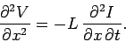 |
(994) |
Differentiating Eq. (993) with respect to yields
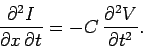 |
(995) |
The above two equations can be combined to give
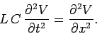 |
(996) |
This is clearly a wave equation, with wave velocity
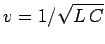 . An
analogous equation can be written for the current,
. An
analogous equation can be written for the current,  .
.
Consider a transmission line which is connected to a generator at one end
( ), and
a resistor,
), and
a resistor,  , at the other (
 ). Suppose that the generator outputs
a voltage
). Suppose that the generator outputs
a voltage
 . If follows that
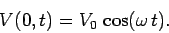 |
(997) |
The solution to the wave equation (996), subject to the above boundary condition, is
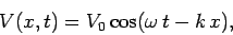 |
(998) |
where  . This clearly corresponds to a wave which propagates
from the generator towards the resistor. Equations (991) and (998) yield
. This clearly corresponds to a wave which propagates
from the generator towards the resistor. Equations (991) and (998) yield
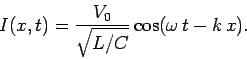 |
(999) |
For self-consistency, the resistor at the end of the line must have a particular
value:
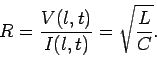 |
(1000) |
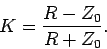
The so-called input impedance of the line is defined
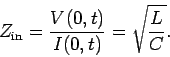 |
(1001) |
Thus, a transmission line terminated by a resistor  acts very
much like a conventional resistor
acts very
much like a conventional resistor
 in the circuit containing
the generator. In fact, the transmission line could be replaced by an effective
resistor
in the circuit diagram for the generator circuit.
The power loss due to this effective resistor corresponds to power which
is extracted from the circuit, transmitted down the line, and absorbed by the
terminating resistor.
in the circuit containing
the generator. In fact, the transmission line could be replaced by an effective
resistor
in the circuit diagram for the generator circuit.
The power loss due to this effective resistor corresponds to power which
is extracted from the circuit, transmitted down the line, and absorbed by the
terminating resistor.
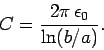
The most commonly occurring type of
transmission line is a co-axial cable, which consists of
two co-axial cylindrical conductors of radii  and
and  (with
(with  ). We
have already shown that the capacitance per unit length of such a cable is
(see Sect. 5.6)
). We
have already shown that the capacitance per unit length of such a cable is
(see Sect. 5.6)
 |
(1002) |
Let us now calculate the inductance per unit length. Suppose that the inner conductor
carries a current . According to Ampère's law, the magnetic field in the
region between the conductors is given by
 |
(1003) |
The flux linking unit length of the cable is
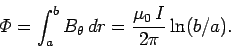 |
(1004) |
Thus, the self-inductance per unit length is
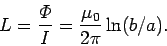 |
(1005) |
So, the speed of propagation of a wave down a co-axial cable is
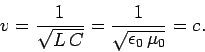 |
(1006) |
Not surprisingly, the wave (which is a type of electromagnetic wave) propagates at
the speed of light. The impedance of the cable is given by
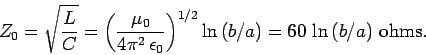 |
(1007) |
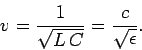
If we fill the region between the two cylindrical conductors with a
dielectric of dielectric constant  , then, according to the
discussion in Sect. 6.2, the capacitance per unit length
of the transmission line goes up by a factor . However,
the dielectric has no effect on magnetic fields, so the inductance
per unit length of the line remains unchanged. It follows that the
propagation speed of signals down a dielectric filled co-axial cable
is
, then, according to the
discussion in Sect. 6.2, the capacitance per unit length
of the transmission line goes up by a factor . However,
the dielectric has no effect on magnetic fields, so the inductance
per unit length of the line remains unchanged. It follows that the
propagation speed of signals down a dielectric filled co-axial cable
is
 |
(1008) |
As we shall see later, this is simply the propagation velocity of electromagnetic waves
through a dielectric medium. The impedance of the cable
becomes
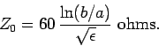 |
(1009) |
We have seen that if a transmission line is terminated by a resistor whose
resistance matches the impedance  of the line then all of the power sent down the
line is absorbed by the resistor. What happens if
of the line then all of the power sent down the
line is absorbed by the resistor. What happens if  ? The answer is
that
some of the power is reflected back down the line. Suppose that the
beginning of the line lies at
? The answer is
that
some of the power is reflected back down the line. Suppose that the
beginning of the line lies at  , and the end of the line is at .
Let us consider a solution
, and the end of the line is at .
Let us consider a solution
![\begin{displaymath}
V(x, t) = V_0 \exp[{\rm i} (\omega t - k x)] + K V_0 \exp[{\rm i} (\omega t + k x)].
\end{displaymath}](img2077.png) |
(1010) |
This corresponds to a voltage wave of amplitude  which travels down the line,
and is reflected at the end of the line, with reflection coefficient
which travels down the line,
and is reflected at the end of the line, with reflection coefficient  .
It is easily demonstrated from the telegrapher's equations that the corresponding
current waveform is
.
It is easily demonstrated from the telegrapher's equations that the corresponding
current waveform is
![\begin{displaymath}
I(x, t) = \frac{V_0}{Z_0} \exp[{\rm i} (\omega t - k x)] - \frac{K V_0}{Z_0}
\exp[{\rm i} (\omega t + k x)].
\end{displaymath}](img2079.png) |
(1011) |
Since the line is terminated by a resistance at , we have, from
Ohm's law,
 |
(1012) |
This yields an expression for the coefficient of reflection,
 |
(1013) |
The input impedance of the line is given by
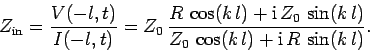 |
(1014) |
Clearly, if the resistor at the end of the line is properly matched, so that
 , then there is no reflection (i.e.,
  ), and the input impedance of
the line is . If the line is short-circuited, so that
), and the input impedance of
the line is . If the line is short-circuited, so that  , then there is total
reflection at the end of the line (i.e.,
, then there is total
reflection at the end of the line (i.e.,  ), and the input impedance becomes
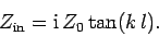 |
(1015) |
This impedance is purely imaginary, implying that the transmission line absorbs no
net power from the generator circuit. In fact, the line acts rather like a pure
inductor or capacitor in the generator circuit
(i.e., it can store, but cannot absorb, energy). If the line
is open-circuited, so that
 , then there is again
total reflection at the end of the line (i.e.,
, then there is again
total reflection at the end of the line (i.e.,  ), and the input
impedance becomes
), and the input
impedance becomes
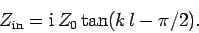 |
(1016) |
Thus, the open-circuited line acts like a closed-circuited line which is shorter by
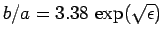
one quarter of a wave-length. For the special case where the length of the line
is exactly one quarter of a wave-length (i.e.,  ), we find
 |
(1017) |
Thus, a quarter-wave line looks like a pure resistor in the generator circuit.
Finally, if the length of the line is much less than the wave-length (i.e.,  )
then we enter the constant-phase regime, and
)
then we enter the constant-phase regime, and
 (i.e., we can
forget about the transmission line connecting the
terminating resistor to the generator circuit).
(i.e., we can
forget about the transmission line connecting the
terminating resistor to the generator circuit).
Suppose that we wish to build a radio transmitter. We can use a standard half-wave antenna (i.e., an antenna whose length is half the wave-length
of the emitted radiation)
to emit the radiation. In electrical circuits, such an antenna acts like a resistor of resistance
73 ohms (it is more usual to say that the antenna has an impedance of 73 ohms--see Sect. 9.2).
Suppose that we buy a 500kW
generator to supply the power to the antenna. How do we transmit
the power from the generator to the antenna? We use a transmission line, of course.
(It is clear that if the distance between the generator and the antenna is of
order the dimensions of the antenna (i.e.,  ) then the constant-phase
approximation breaks down, and so we have to use a transmission line.)
Since the impedance of the antenna is fixed at 73 ohms, we need to use a
73 ohm transmission line (i.e.,
) then the constant-phase
approximation breaks down, and so we have to use a transmission line.)
Since the impedance of the antenna is fixed at 73 ohms, we need to use a
73 ohm transmission line (i.e.,  ohms) to connect the generator to
the antenna, otherwise some of the power we send down the line is reflected
(i.e., not all of the power output of the generator is converted into
radio waves). If we wish to use a co-axial cable to connect the generator to
the antenna, then it is clear from Eq. (1009) that the radii of the
inner and outer conductors need to be such that
ohms) to connect the generator to
the antenna, otherwise some of the power we send down the line is reflected
(i.e., not all of the power output of the generator is converted into
radio waves). If we wish to use a co-axial cable to connect the generator to
the antenna, then it is clear from Eq. (1009) that the radii of the
inner and outer conductors need to be such that
 .
.
Suppose, finally, that we upgrade our transmitter to use a full-wave antenna
(i.e., an antenna whose length equals the wave-length of the emitted radiation).
A full-wave antenna has a different impedance than a half-wave antenna. Does
this mean that we have to rip out our original co-axial cable, and replace it
by one whose impedance matches that of the new antenna? Not necessarily.
Let be the impedance of the co-axial cable, and  the impedance of
the antenna. Suppose that we place a quarter-wave transmission line (i.e., one whose
length is one quarter of a wave-length) of characteristic
impedance
the impedance of
the antenna. Suppose that we place a quarter-wave transmission line (i.e., one whose
length is one quarter of a wave-length) of characteristic
impedance
 between the end of the cable and the
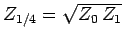
antenna. According to Eq. (1017) (with
between the end of the cable and the
antenna. According to Eq. (1017) (with
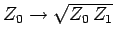 and
and
 ), the input impedance of the quarter-wave line
is
), the input impedance of the quarter-wave line
is
 , which matches that of the cable. The output impedance
matches that of the antenna. Consequently, there is no reflection of the power
sent down the cable to the antenna. A quarter-wave line of the appropriate impedance
can easily
be fabricated from a short length of co-axial cable of the appropriate
, which matches that of the cable. The output impedance
matches that of the antenna. Consequently, there is no reflection of the power
sent down the cable to the antenna. A quarter-wave line of the appropriate impedance
can easily
be fabricated from a short length of co-axial cable of the appropriate  .
.
Next: Electromagnetic energy and momentum
Up: Magnetic induction
Previous: Alternating current circuits
Richard Fitzpatrick
2006-02-02