Potential formulation

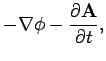
We have seen that Eqs. (418) and (419) are automatically satisfied if we write the electric and magnetic fields in terms of potentials:

$${\bf E} = - \nabla\phi - \frac{\partial {\bf A}}{\partial t},$$ (421)

$${\bf B} = \nabla\times{\bf A}.$$ (422)

This prescription is not unique, but we can make it unique by adopting the following conventions:

$$\phi({\bf r}) \rightarrow 0\mbox{\hspace{0.5cm}as   $\vert{\bf r}\vert \rightarrow \infty$},$$ (423)

$$\nabla\cdot {\bf A} = -\epsilon_0 \mu_0 \frac{\partial \phi}{\partial t}.$$ (424)

The above equations can be combined with Eq. (417) to give

$$\epsilon_0\mu_0 \frac{\partial^2\phi}{\partial t^2} - \nabla^2\phi = \frac{\rho} {\epsilon_0}.$$ (425)

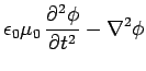
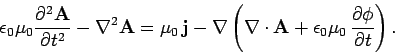
Let us now consider Eq. (420). Substitution of Eqs. (421) and (422) into this formula yields

$$\nabla\times\nabla\times {\bf A} \equiv \nabla(\nabla\cdot{\... ...} - \epsilon_0\mu_0 \frac{\partial^2 {\bf A}}{\partial t^2},$$ (426)

or

$$\epsilon_0 \mu_0 \frac{\partial^2 {\bf A}}{\partial t^2} - \... ...A} +\epsilon_0\mu_0 \frac{\partial\phi} {\partial t}\right).$$ (427)

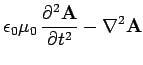
We can now see quite clearly where the Lorentz gauge condition (398) comes from. The above equation is, in general, very complicated, since it involves both the vector and scalar potentials. But, if we adopt the Lorentz gauge, then the last term on the right-hand side becomes zero, and the equation simplifies considerably, such that it only involves the vector potential. 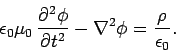Thus, we find that Maxwell's equations reduce to the following:

$$\epsilon_0\mu_0 \frac{\partial^2\phi}{\partial t^2} - \nabla^2\phi = \frac{\rho}{\epsilon_0},$$ (428)

$$\epsilon_0\mu_0 \frac{\partial^2{\bf A} }{\partial t^2} - \nabla^2{\bf A} = \mu_0 {\bf j}.$$ (429)

This is the same (scalar) equation written four times over. In steady-state (i.e., $\partial/\partial t=0$), it reduces to Poisson's equation, which we know how to solve. With the $\partial^2/\partial t^2$ terms included, it becomes a slightly more complicated equation (in fact, a driven three-dimensional wave equation).