Next: Euler's equations Up: Rigid body rotation Previous: Rotational kinetic energy
 , defined in Section 8.3, takes the form of a real symmetric
  matrix. It therefore follows, from the standard matrix theory discussed in Section A.11,
that the moment of inertia tensor possesses three mutually orthogonal eigenvectors which are associated with three real eigenvalues. Let the
matrix. It therefore follows, from the standard matrix theory discussed in Section A.11,
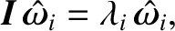
that the moment of inertia tensor possesses three mutually orthogonal eigenvectors which are associated with three real eigenvalues. Let the  th eigenvector (which can be normalized to
be a unit vector) be denoted
th eigenvector (which can be normalized to
be a unit vector) be denoted
 , and the th eigenvalue
  . It then
follows that
for
. It then
follows that
for 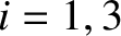 .
.
The directions of the three mutually orthogonal unit vectors
define the three so-called principal axes
of rotation of the rigid body under investigation. These axes are special because when the body rotates about
one of them (i.e., when
 is parallel to one of them) the angular momentum vector
  becomes parallel to the angular velocity vector
.
This can be seen from a comparison of Equation (8.13) and Equation (8.19).
becomes parallel to the angular velocity vector
.
This can be seen from a comparison of Equation (8.13) and Equation (8.19).
Suppose that we reorient our Cartesian coordinate
axes so they coincide with the mutually orthogonal principal axes of rotation. In this new reference frame, the eigenvectors of
are the unit vectors,
 ,
,  , and
, and  , and the eigenvalues
are the moments of inertia about these axes,
, and the eigenvalues
are the moments of inertia about these axes,
 ,
,
 , and
, and
 , respectively. These latter quantities are referred to as the
principal moments of inertia.
The products of inertia are all zero in the new
reference frame. Hence, in this frame, the moment
of inertia tensor takes the form of a diagonal matrix:
, respectively. These latter quantities are referred to as the
principal moments of inertia.
The products of inertia are all zero in the new
reference frame. Hence, in this frame, the moment
of inertia tensor takes the form of a diagonal matrix:
 |
(8.20) |
, , and are indeed
the eigenvectors of this matrix, with the eigenvalues
,
, and
, respectively, and that
 is indeed parallel to
whenever
is directed along , , or .
is indeed parallel to
whenever
is directed along , , or .
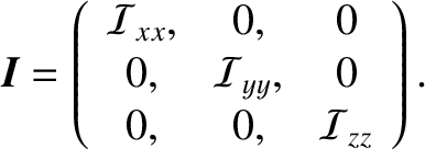
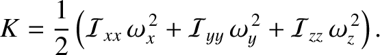
When expressed in our new coordinate system, Equation (8.13) yields
 |
(8.21) |
 |
(8.22) |
In conclusion, there are many great simplifications to be had by choosing a coordinate system whose axes coincide with the principal axes of rotation of the rigid body under investigation.